Flux

This article is about the concept of flux in natural science and mathematics. For other uses, see Flux (disambiguation).

The field lines of a vector field F through surfaces with unit normal n, the angle from n to F is θ. Flux is a measure of how much of the field passes through a given surface. F is decomposed into components perpendicular (⊥) and parallel ( ‖ ) to n. Only the parallel component contributes to flux because it is the maximum extent of the field passing through the surface at a point, the perpendicular component does not contribute. Top: Three field lines through a plane surface, one normal to the surface, one parallel, and one intermediate. Bottom: Field line through a curved surface, showing the setup of the unit normal and surface element to calculate flux.

Flux is either of two separate simple and ubiquitous concepts throughout physics and applied mathematics. Within a discipline, the term is generally used consistently, but care must be taken when comparing phenomena from different disciplines. Both concepts have mathematical rigor, enabling comparison of the underlying math when the terminology is unclear. For transport phenomena, flux is a vector quantity, describing the magnitude and direction of the flow of a substance or property. In electromagnetism, flux is a scalar quantity, defined as the surface integral of the component of a vector field perpendicular to the surface at each point. As will be made clear, the easiest way to relate the two concepts is that the surface integral of a flux according to the first definition is a flux according to the second definition.

Terminology

The word flux comes from Latin: fluxus means "flow", and fluere is "to flow".^[1] As fluxion, this term was introduced into differential calculus by Isaac Newton.

One could argue, based on the work of James Clerk Maxwell,^[2] that the transport definition precedes the way the term is used in electromagnetism. The specific quote from Maxwell is:

In the case of fluxes, we have to take the integral, over a surface, of the flux through every element of the surface. The result of this operation is called the surface integral of the flux. It represents the quantity which passes through the surface.
— James Clerk Maxwell

According to the first definition, flux may be a single vector, or flux may be a vector field / function of position. In the latter case flux can readily be integrated over a surface. By contrast, according to the second definition, flux is the integral over a surface; it makes no sense to integrate a second-definition flux for one would be integrating over a surface twice. Thus, Maxwell's quote only makes sense if "flux" is being used according to the first definition (and furthermore is a vector field rather than single vector). This is ironic because Maxwell was one of the major developers of what we now call "electric flux" and "magnetic flux" according to the second definition. Their names in accordance with the quote (and first definition) would be "surface integral of electric flux" and "surface integral of magnetic flux", in which case "electric flux" would instead be defined as "electric field" and "magnetic flux" defined as "magnetic field". This implies that Maxwell conceived as these fields as flows/fluxes of some sort.

Given a flux according to the second definition, the corresponding flux density, if that term is used, refers to its derivative along the surface that was integrated. By the Fundamental theorem of calculus, the corresponding flux density is a flux according to the first definition. Given a current such as electric current—charge per time, current density would also be a flux according to the first definition—charge per time per area. Due to the conflicting definitions of flux, and the interchangeability of flux, flow, and current in nontechnical English, all of the terms used in this paragraph are sometimes used interchangeably and ambiguously. Concrete fluxes in the rest of this article will be used in accordance to their broad acceptance in the literature, regardless of which definition of flux the term corresponds to.

Flux as flow rate per unit area

In transport phenomena (heat transfer, mass transfer and fluid dynamics), flux is defined as the rate of flow of a property per unit area, which has the dimensions [quantity]·[time]⁻¹·[area]⁻¹.^[3] The area is of the surface the property is flowing "through" or "across". For example, the magnitude of a river's current, i.e. the amount of water that flows through a cross-section of the river each second, or the amount of sunlight that lands on a patch of ground each second, are kinds of flux.

General mathematical definition (transport)

Here are 3 definitions in increasing order of complexity. Each is a special case of the following. In all cases the frequent symbol j, (or J) is used for flux, q for the physical quantity that flows, t for time, and A for area. These identifiers will be written in bold when and only when they are vectors.

First, flux as a (single) scalar:

j={\frac {I}{A}}

where:

I=\lim \limits _{\Delta t\rightarrow 0}{\frac {\Delta q}{\Delta t}}={\frac {\mathrm {d} q}{\mathrm {d} t}}

In this case the surface in which flux is being measured is fixed, and has area A. The surface is assumed to be flat, and the flow is assumed to be everywhere constant with respect to position, and perpendicular to the surface.

Second, flux as a scalar field defined along a surface, i.e. a function of points on the surface:

j(\mathbf {p} )={\frac {\partial I}{\partial A}}(\mathbf {p} )

I(A,\mathbf {p} )={\frac {\mathrm {d} q}{\mathrm {d} t}}(A,\mathbf {p} )

As before, the surface is assumed to be flat, and the flow is assumed to be everywhere perpendicular to it. However the flow need not be constant. q is now a function of p, a point on the surface, and A, an area. Rather than measure the total flow through the surface, q measures the flow through the disk with area A centered at p along the surface.

Finally, flux as a vector field:

\mathbf {j} (\mathbf {p} )={\frac {\partial \mathbf {I} }{\partial A}}(\mathbf {p} )

\mathbf {I} (A,\mathbf {p} )={\underset {\mathbf {\hat {n}} }{\operatorname {arg\,max} }}\,\mathbf {\hat {n}} _{\mathbf {p} }{\frac {\mathrm {d} q}{\mathrm {d} t}}(A,\mathbf {p} ,\mathbf {\hat {n}} )

In this case, there is no fixed surface we are measuring over. q is a function of a point, an area, and a direction (given by a unit vector, $\mathbf {\hat {n}}$ ), and measures the flow through the disk of area A perpendicular to that unit vector. I is defined picking the unit vector that maximizes the flow around the point, because the true flow is maximized across the disk that is perpendicular to it. The unit vector thus uniquely maximizes the function when it points in the "true direction" of the flow. [Strictly speaking, this is an abuse of notation because the "arg max" cannot directly compare vectors; we take the vector with the biggest norm instead.]

Properties

These direct definition, especially the last, are rather unwieldy. For example, the argmax construction is artificial from the perspective of empirical measurements, when with a Weathervane or similar one can easily deduce the direction of flux at a point. Rather than defining the vector flux directly, it is often more intuitive to state some properties about it. Furthermore, from these properties the flux can uniquely be determined anyway.

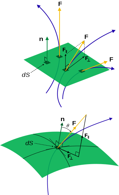
If the flux j passes through the area at an angle θ to the area normal $\mathbf {\hat {n}}$ , then

\mathbf {j} \cdot \mathbf {\hat {n}} =j\cos \theta

where · is the dot product of the unit vectors. This is, the component of flux passing through the surface (i.e. normal to it) is j cos θ, while the component of flux passing tangential to the area is j sin θ, but there is no flux actually passing through the area in the tangential direction. The only component of flux passing normal to the area is the cosine component.

For vector flux, the surface integral of j over a surface S, gives the proper flowing per unit of time through the surface.

{\frac {\mathrm {d} q}{\mathrm {d} t}}=\iint _{S}\mathbf {j} \cdot \mathbf {\hat {n}} \,{\rm {d}}A\ =\iint _{S}\mathbf {j} \cdot {\rm {d}}\mathbf {A}

A (and its infinitesimal) is the vector area, combination of the magnitude of the area through which the property passes through, A, and a unit vector normal to the area, $\mathbf {\hat {n}}$ . The relation is $\mathbf {A} =A\mathbf {\hat {n}}$ . Unlike in the second set of equations, the surface here need not be flat.

Finally, we can integrate again over the time duration t₁ to t₂, getting the total amount of the property flowing through the surface in that time (t₂ − t₁):

q=\int _{t_{1}}^{t_{2}}\iint _{S}\mathbf {j} \cdot {\rm {d}}{\mathbf {A} }\,{\rm {d}}t

Transport fluxes

Eight of the most common forms of flux from the transport phenomena literature are defined as follows:

Momentum flux, the rate of transfer of momentum across a unit area (N·s·m⁻²·s⁻¹). (Newton's law of viscosity)^[4]
Heat flux, the rate of heat flow across a unit area (J·m⁻²·s⁻¹). (Fourier's law of conduction)^[5] (This definition of heat flux fits Maxwell's original definition.)^[2]
Diffusion flux, the rate of movement of molecules across a unit area (mol·m⁻²·s⁻¹). (Fick's law of diffusion)^[4]
Volumetric flux, the rate of volume flow across a unit area (m³·m⁻²·s⁻¹). (Darcy's law of groundwater flow)
Mass flux, the rate of mass flow across a unit area (kg·m⁻²·s⁻¹). (Either an alternate form of Fick's law that includes the molecular mass, or an alternate form of Darcy's law that includes the density.)
Radiative flux, the amount of energy transferred in the form of photons at a certain distance from the source per unit area per second (J·m⁻²·s⁻¹). Used in astronomy to determine the magnitude and spectral class of a star. Also acts as a generalization of heat flux, which is equal to the radiative flux when restricted to the infrared spectrum.
Energy flux, the rate of transfer of energy through a unit area (J·m⁻²·s⁻¹). The radiative flux and heat flux are specific cases of energy flux.
Particle flux, the rate of transfer of particles through a unit area ([number of particles] m⁻²·s⁻¹)

These fluxes are vectors at each point in space, and have a definite magnitude and direction. Also, one can take the divergence of any of these fluxes to determine the accumulation rate of the quantity in a control volume around a given point in space. For incompressible flow, the divergence of the volume flux is zero.

Chemical diffusion

As mentioned above, chemical molar flux of a component A in an isothermal, isobaric system is defined in Fick's law of diffusion as:

\mathbf {J} _{A}=-D_{AB}\nabla c_{A}

where the nabla symbol ∇ denotes the gradient operator, D_AB is the diffusion coefficient (m²·s⁻¹) of component A diffusing through component B, c_A is the concentration (mol/m³) of component A.^[6]

This flux has units of mol·m⁻²·s⁻¹, and fits Maxwell's original definition of flux.^[2]

For dilute gases, kinetic molecular theory relates the diffusion coefficient D to the particle density n = N/V, the molecular mass m, the collision cross section $\sigma$ , and the absolute temperature T by

D={\frac {2}{3n\sigma }}{\sqrt {\frac {kT}{\pi m}}}

where the second factor is the mean free path and the square root (with Boltzmann's constant k) is the mean velocity of the particles.

In turbulent flows, the transport by eddy motion can be expressed as a grossly increased diffusion coefficient.

Quantum mechanics

Main article: Probability current

In quantum mechanics, particles of mass m in the quantum state ψ(r, t) have a probability density defined as

\rho =\psi ^{*}\psi =|\psi |^{2}.\,

So the probability of finding a particle in a differential volume element d³r is

{\rm {d}}P=|\psi |^{2}{\rm {d}}^{3}\mathbf {r} .\,

Then the number of particles passing perpendicularly through unit area of a cross-section per unit time is the probability flux;

\mathbf {J} ={\frac {i\hbar }{2m}}\left(\psi \nabla \psi ^{*}-\psi ^{*}\nabla \psi \right).\,

This is sometimes referred to as the probability current or current density,^[7] or probability flux density.^[8]

Flux as a surface integral

The flux visualized. The rings show the surface boundaries. The red arrows stand for the flow of charges, fluid particles, subatomic particles, photons, etc. The number of arrows that pass through each ring is the flux.

General mathematical definition (surface integral)

As a mathematical concept, flux is represented by the surface integral of a vector field,^[9]

\Phi _{F}=\iint _{A}\mathbf {F} \cdot \mathrm {d} \mathbf {A}

where F is a vector field, and dA is the vector area of the surface A, directed as the surface normal.

The surface has to be orientable, i.e. two sides can be distinguished: the surface does not fold back onto itself. Also, the surface has to be actually oriented, i.e. we use a convention as to flowing which way is counted positive; flowing backward is then counted negative.

The surface normal is usually directed by the right-hand rule.

Conversely, one can consider the flux the more fundamental quantity and call the vector field the flux density.

Often a vector field is drawn by curves (field lines) following the "flow"; the magnitude of the vector field is then the line density, and the flux through a surface is the number of lines. Lines originate from areas of positive divergence (sources) and end at areas of negative divergence (sinks).

See also the image at right: the number of red arrows passing through a unit area is the flux density, the curve encircling the red arrows denotes the boundary of the surface, and the orientation of the arrows with respect to the surface denotes the sign of the inner product of the vector field with the surface normals.

If the surface encloses a 3D region, usually the surface is oriented such that the influx is counted positive; the opposite is the outflux.

The divergence theorem states that the net outflux through a closed surface, in other words the net outflux from a 3D region, is found by adding the local net outflow from each point in the region (which is expressed by the divergence).

If the surface is not closed, it has an oriented curve as boundary. Stokes' theorem states that the flux of the curl of a vector field is the line integral of the vector field over this boundary. This path integral is also called circulation, especially in fluid dynamics. Thus the curl is the circulation density.

We can apply the flux and these theorems to many disciplines in which we see currents, forces, etc., applied through areas.

Electromagnetism

One way to better understand the concept of flux in electromagnetism is by comparing it to a butterfly net. The amount of air moving through the net at any given instant in time is the flux. If the wind speed is high, then the flux through the net is large. If the net is made bigger, then the flux is larger even though the wind speed is the same. For the most air to move through the net, the opening of the net must be facing the direction the wind is blowing. If the net is parallel to the wind, then no wind will be moving through the net. The simplest way to think of flux is "how much air goes through the net", where the air is a velocity field and the net is the boundary of an imaginary surface.

Electric flux

Two forms of electric flux are used, one for the E-field:^[10]^[11]

\Phi _{E}=

$\oiint$

{\scriptstyle A}

\mathbf {E} \cdot {\rm {d}}\mathbf {A}

and one for the D-field (called the electric displacement):

\Phi _{D}=

$\oiint$

{\scriptstyle A}

\mathbf {D} \cdot {\rm {d}}\mathbf {A}

This quantity arises in Gauss's law – which states that the flux of the electric field E out of a closed surface is proportional to the electric charge Q_A enclosed in the surface (independent of how that charge is distributed), the integral form is:

$\oiint$

{\scriptstyle A}

\mathbf {E} \cdot {\rm {d}}\mathbf {A} ={\frac {Q_{A}}{\varepsilon _{0}}}

where ε₀ is the permittivity of free space.

If one considers the flux of the electric field vector, E, for a tube near a point charge in the field the charge but not containing it with sides formed by lines tangent to the field, the flux for the sides is zero and there is an equal and opposite flux at both ends of the tube. This is a consequence of Gauss's Law applied to an inverse square field. The flux for any cross-sectional surface of the tube will be the same. The total flux for any surface surrounding a charge q is q/ε₀.^[12]

In free space the electric displacement is given by the constitutive relation D = ε₀ E, so for any bounding surface the D-field flux equals the charge Q_A within it. Here the expression "flux of" indicates a mathematical operation and, as can be seen, the result is not necessarily a "flow", since nothing actually flows along electric field lines.

Magnetic flux

The magnetic flux density (magnetic field) having the unit Wb/m² (Tesla) is denoted by B, and magnetic flux is defined analogously:^[10]^[11]

\Phi _{B}=

$\oiint$

{\scriptstyle A}

\mathbf {B} \cdot {\rm {d}}\mathbf {A}

with the same notation above. The quantity arises in Faraday's law of induction, in integral form:

\oint _{C}\mathbf {E} \cdot d{\boldsymbol {\ell }}=-\int _{\partial C}{\partial \mathbf {B} \over \partial t}\cdot {\rm {d}}\mathbf {s} =-{\frac {{\rm {d}}\Phi _{B}}{{\rm {d}}t}}

where dℓ is an infinitesimal vector line element of the closed curve C, with magnitude equal to the length of the infinitesimal line element, and direction given by the tangent to the curve C, with the sign determined by the integration direction.

The time-rate of change of the magnetic flux through a loop of wire is minus the electromotive force created in that wire. The direction is such that if current is allowed to pass through the wire, the electromotive force will cause a current which "opposes" the change in magnetic field by itself producing a magnetic field opposite to the change. This is the basis for inductors and many electric generators.

Poynting flux

Using this definition, the flux of the Poynting vector S over a specified surface is the rate at which electromagnetic energy flows through that surface, defined like before:^[11]

\Phi _{S}=

$\oiint$

{\scriptstyle A}

\mathbf {S} \cdot {\rm {d}}\mathbf {A}

The flux of the Poynting vector through a surface is the electromagnetic power, or energy per unit time, passing through that surface. This is commonly used in analysis of electromagnetic radiation, but has application to other electromagnetic systems as well.

Confusingly, the Poynting vector is sometimes called the power flux, which is an example of the first usage of flux, above.^[13] It has units of watts per square metre (W/m²).

Notes

↑ Weekley, Ernest (1967). An Etymological Dictionary of Modern English. Courier Dover Publications. p. 581. ISBN 0-486-21873-2.
1 2 3 Maxwell, James Clerk (1892). Treatise on Electricity and Magnetism. ISBN 0-486-60636-8.
↑ Bird, R. Byron; Stewart, Warren E.; Lightfoot, Edwin N. (1960). Transport Phenomena. Wiley. ISBN 0-471-07392-X.
1 2 P.M. Whelan; M.J. Hodgeson (1978). Essential Principles of Physics (2nd ed.). John Murray. ISBN 0-7195-3382-1.
↑ Carslaw, H.S.; Jaeger, J.C. (1959). Conduction of Heat in Solids (Second ed.). Oxford University Press. ISBN 0-19-853303-9.
↑ Welty; Wicks, Wilson and Rorrer (2001). Fundamentals of Momentum, Heat, and Mass Transfer (4th ed.). Wiley. ISBN 0-471-38149-7.
↑ D. McMahon (2006). Quantum Mechanics Demystified. Demystified. Mc Graw Hill. ISBN 0-07-145546-9.
↑ Sakurai, J. J. (1967). Advanced Quantum Mechanics. Addison Wesley. ISBN 0-201-06710-2.
↑ M.R. Spiegel; S. Lipcshutz; D. Spellman (2009). Vector Analysis. Schaum's Outlines (2nd ed.). McGraw Hill. p. 100. ISBN 978-0-07-161545-7.
1 2 I.S. Grant; W.R. Phillips (2008). Electromagnetism. Manchester Physics (2nd ed.). John Wiley & Sons. ISBN 978-0-471-92712-9.
1 2 3 D.J. Griffiths (2007). Introduction to Electrodynamics (3rd ed.). Pearson Education, Dorling Kindersley. ISBN 81-7758-293-3.
↑ Feynman, Richard P (1964). The Feynman Lectures on Physics. II. Addison-Wesley. pp. 4–8, 9. ISBN 0-7382-0008-5.
↑ Wangsness, Roald K. (1986). Electromagnetic Fields (2nd ed.). Wiley. ISBN 0-471-81186-6. p.357

External links

The dictionary definition of flux at Wiktionary

This article is issued from Wikipedia - version of the 10/4/2016. The text is available under the Creative Commons Attribution/Share Alike but additional terms may apply for the media files.

Flux

Terminology

Flux as flow rate per unit area

General mathematical definition (transport)

Properties

Transport fluxes

Chemical diffusion

Quantum mechanics

Flux as a surface integral

General mathematical definition (surface integral)

Electromagnetism

Electric flux

Magnetic flux

Poynting flux

See also

Notes

Further reading

External links