Exponential distribution

Not to be confused with the exponential family of probability distributions.

Exponential
Probability density function
Cumulative distribution function
Parameters	λ > 0 rate, or inverse scale
Support	x ∈ [0, ∞)
PDF	λ e^−λx
CDF	1 − e^−λx
Quantile	−ln(1 − F) / λ
Mean	λ⁻¹ (= β)
Median	λ⁻¹ ln(2)
Mode	0
Variance	λ⁻² (= β²)
Skewness	2
Ex. kurtosis	6
Entropy	1 − ln(λ)
MGF	$\frac{\lambda}{\lambda-t}, \text{ for } t < \lambda$
CF	$\frac{\lambda}{\lambda-it}$
Fisher information	$\lambda^{-2}$

In probability theory and statistics, the exponential distribution (a.k.a. negative exponential distribution) is the probability distribution that describes the time between events in a Poisson process, i.e. a process in which events occur continuously and independently at a constant average rate. It is a particular case of the gamma distribution. It is the continuous analogue of the geometric distribution, and it has the key property of being memoryless. In addition to being used for the analysis of Poisson processes, it is found in various other contexts.

The exponential distribution is not the same as the class of exponential families of distributions, which is a large class of probability distributions that includes the exponential distribution as one of its members, but also includes the normal distribution, binomial distribution, gamma distribution, Poisson, and many others.

Introduction to the exponential distribution

The exponential distribution is used to model the time between the occurrence of events in an interval of time, or the distance between events in space. The exponential distribution may be useful to model events such as

The time between goals scored in a World Cup soccer match
The time between customer calls to a help center^[1]
The time between meteors greater than 1 meter diameter striking earth
The time between successive failures of a machine
The time from diagnosis until death in patients with metastatic cancer
The distance between successive breaks in a pipeline

The exponential distribution is an appropriate model if the following conditions are true.

X is the time (or distance) between events, with X > 0.
The occurrence of one event does not affect the probability that a second event will occur. That is, events occur independently.
The rate at which events occur is constant. The rate cannot be higher in some intervals and lower in other intervals.
Two events cannot occur at exactly the same instant.

If these conditions are true, then X is an exponential random variable, and the distribution of X is an exponential distribution. If these conditions are not true, then the exponential distribution is not appropriate. Alternative distributions such as the Weibull or gamma may give a better fit to the data, or a semi-parametric model, such as the Cox proportional-hazards model, may be required for statistical analysis.

The graph of an exponential distribution starts on the y-axis at a positive value (called lambda, λ) and decreases to the right.

Graph of exponential distribution PDF with λ = 1

The exponential distribution is specified by the single parameter lambda (λ). Lambda is the event rate, and may have different names in other applications:

event rate
rate parameter
arrival rate
death rate
failure rate
transition rate

Lambda is the number of events per unit time. The graph of the exponential distribution, called the probability density function (PDF), shows the distribution of time (or distance) between events. The PDF is specified in terms of lambda (events per unit time) and x (time).

{\text{density}}=f(x)=\lambda e^{-\lambda x}

where

λ is the rate parameter
x > 0
e is the number 2.71828 …, the base of the natural logs

The density f(x) is 0 for x less than or equal to 0.

The figure shows the PDF for exponential distributions with λ = 1, 2, 3, and 0.5. The line for each distribution meets the y-axis at lambda. Notice in the figure that when lambda (the event rate) is large, the time between events is small. In particular, the mean time between events is given by 1/λ. For λ = 3, the mean time between events is 1/λ = 1/3. For λ = 0.5, the mean time between events is 1/λ = 1/0.5 = 2.

Olkin ^[2] gives the following example of data modeled using an exponential distribution. The time between successive failures of the air-conditioning system of a particular jet airplane were recorded:

Time between successive failures = 23, 261, 87, 7, 120, 14, 62, 47, 225, 71, 246, 21, 42, 20, 5, 12, 120, 11, 3, 14, 71, 11, 14, 11, 16, 90, 1, 16, 52, 95

The mean time between failures is 59.6. The median time between failures is 22. Because the exponential distribution is skewed right, the median is less than the mean. The figure shows a histogram of the time between failures and a fitted exponential density curve with λ = 1/(mean time to failure) = 1/59.6 = 0.0168.

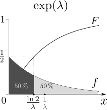
Cumulative distribution function

The probability that the time between events is less than a specified time x is given by the cumulative distribution function (CDF):

P({\text{time between events is}}\leq \ x)=1-e^{(-\lambda x)}

The figures below show the probability density and cumulative distribution functions for the exponential distribution with lambda = 1.

Examples using the CDF to calculate probability

Example 1. The time between failures in the air-conditioner example was modelled as an exponential distribution with lambda = 0.0168. For λ = 0.0168, the mean time between failures is 1/0.0168 = 59.5 hours. What is the probability that the time until the next failure is less than 100 hours? This question can be answered using the cumulative distribution function. The graph shows the CDF for this example.

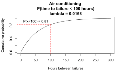
The graph shows that, using the cumulative distribution function with λ = 0.0168, the value of x = 100 corresponds to a value of y = 0.81. So the probability that the time until the next failure is less than 100 hours is p = 0.81. The same probability can be calculated using the formula for the CDF:

P(time between events is < x) = 1 − e^(−λx)

P(time between events is < 100)=1-e^(-0.0168×100) = 0.8136

Example 2. For an exponential distribution with λ = 4, what is the probability that the time between events (x) is less than 0.5?

From the equation for the CDF, P(time between events is < 0.5) = 1 − e^(-4·0.5) = 0.865

This probability may also be visualized by examining the PDF and CDF, which show that 86.5% of the area under the curve is less than x = 0.5.

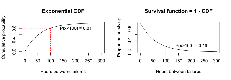
Exponential distribution in survival analysis

In survival analysis, the exponential distribution can be used to model the distribution of survival times for subjects in the study. The survivor function is the probability that a subject survives longer than time x. Because the CDF is the probability that a subject survives less than time x, the survivor function = 1 − CDF.

P(time between events is > 100) = 1 − P(time between events is < 100) = 1 − (1 − e^−λx) ) = e^−λx)

The CDF graph below for the air conditioner failure example shows that P(x < 100) = 0.81. The survivor function graph shows that P(x > 100) = 1 − P(x < 100) = 1 – 0.81 = 0.19.

Examples that violate the assumptions of an exponential distribution

The time between arrivals of students at the student union will likely not follow an exponential distribution, because the rate is not constant (low rate during class time, high rate between class times) and the arrivals of individual students are not independent (students tend to come in groups).

The time between magnitude 5 earthquakes per year in California may not follow an exponential distribution, if one large earthquake increases the probability of aftershocks of similar magnitude.

While the exponential distribution is sometimes appropriate to model survival, the actual distribution of lifespans in many settings do not follow the exponential distribution. In these situations, the Weibull or gamma distribution is commonly used, particularly for machines or devices. In medical research, survival is most commonly modeled using non-parametric or semi-parametric methods such as the Kaplan-Meier plot and Cox proportional hazards regression, rather than with parametric distributions such as the exponential or Weibull.

The graph shows a distribution of event times that is not exponential. The data are the age at first marriage of 5,534 US women who responded to the National Survey of Family Growth (NSFG) conducted by the CDC in the 2006 and 2010 cycle, from the data set ageAtMar in the R package openintro. In the example, the event is first marriage, and the time to event is age.

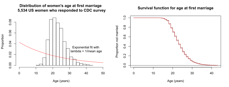
These data violate the requirement that the rate at which events occur is constant. In these data, the rate is much higher in some intervals and lower in other intervals. The red line on the histogram shows the exponential curve fitted with lambda = 1/mean age. The survivor function graph is on the right and includes the 95% confidence interval in red. The survivor function and fitted exponential curve show that the decline from the initial value is not exponential.

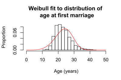
The figure shows a Weibull distribution fit to the age at first marriage. While not a perfect fit, it is superior to the exponential fit, and would be more appropriate for modelling age at first marriage.

Characterization

Probability density function

The probability density function (pdf) of an exponential distribution is

f(x;\lambda) = \begin{cases} \lambda e^{-\lambda x} & x \ge 0, \\ 0 & x < 0. \end{cases}

Alternatively, this can be defined using the right-continuous Heaviside step function, H(x) where H(0)=1:

f(x;\lambda) = \mathrm \lambda e^{-\lambda x} H(x)

Here λ > 0 is the parameter of the distribution, often called the rate parameter. The distribution is supported on the interval [0, ∞). If a random variable X has this distribution, we write X ~ Exp(λ).

The exponential distribution exhibits infinite divisibility.

Cumulative distribution function

The cumulative distribution function is given by

F(x;\lambda) = \begin{cases} 1-e^{-\lambda x} & x \ge 0, \\ 0 & x < 0. \end{cases}

Alternatively, this can be defined using the Heaviside step function, H(x).

F(x;\lambda) = \mathrm (1-e^{-\lambda x}) H(x)

Alternative parameterization

A commonly used alternative parametrization is to define the probability density function (pdf) of an exponential distribution as

f(x;\beta) = \begin{cases} \frac{1}{\beta} e^{-\frac{x}{\beta}} & x \ge 0, \\ 0 & x < 0. \end{cases}

where β > 0 is mean, standard deviation, and scale parameter of the distribution, the reciprocal of the rate parameter, λ, defined above. In this specification, β is a survival parameter in the sense that if a random variable X is the duration of time that a given biological or mechanical system manages to survive and X ~ Exp(β) then E[X] = β. That is to say, the expected duration of survival of the system is β units of time. The parametrization involving the "rate" parameter arises in the context of events arriving at a rate λ, when the time between events (which might be modeled using an exponential distribution) has a mean of β = λ⁻¹.

The alternative specification is sometimes more convenient than the one given above, and some authors will use it as a standard definition. This alternative specification is not used here. Unfortunately this gives rise to a notational ambiguity. In general, the reader must check which of these two specifications is being used if an author writes "X ~ Exp(λ)", since either the notation in the previous (using λ) or the notation in this section (here, using β to avoid confusion) could be intended. An example of this notational switch: reference^[3] uses λ for β.

Properties

Mean, variance, moments and median

The mean is the probability mass centre, that is the first moment.

The median is the preimage F⁻¹(1/2).

The mean or expected value of an exponentially distributed random variable X with rate parameter λ is given by

\operatorname{E}[X] = \frac{1}{\lambda} = \beta

, see above.

In light of the examples given above, this makes sense: if you receive phone calls at an average rate of 2 per hour, then you can expect to wait half an hour for every call.

The variance of X is given by

\operatorname{Var}[X] = \frac{1}{\lambda^2}

so the standard deviation is equal to the mean.

The moments of X, for n = 1, 2, ..., are given by

\operatorname{E}\left [X^n \right ] = \frac{n!}{\lambda^n}

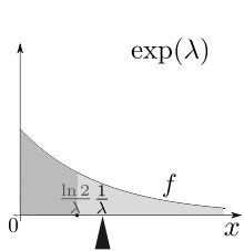
The median of X is given by

\operatorname{m}[X] = \frac{\ln(2)}{\lambda} < \operatorname{E}[X]

where ln refers to the natural logarithm. Thus the absolute difference between the mean and median is

|\operatorname{E}[X]- \operatorname{m}[X]| = \frac{1- \ln(2)}{\lambda}< \frac{1}{\lambda} = \text{standard deviation}

in accordance with the median-mean inequality.

Memorylessness

An exponentially distributed random variable T obeys the relation

\Pr \left (T > s + t | T > s \right ) = \Pr(T > t), \qquad \forall s, t \ge 0

When T is interpreted as the waiting time for an event to occur relative to some initial time, this relation implies that, if T is conditioned on a failure to observe the event over some initial period of time s, the distribution of the remaining waiting time is the same as the original unconditional distribution. For example, if an event has not occurred after 30 seconds, the conditional probability that occurrence will take at least 10 more seconds is equal to the unconditional probability of observing the event more than 10 seconds relative to the initial time.

The exponential distribution and the geometric distribution are the only memoryless probability distributions.

The exponential distribution is consequently also necessarily the only continuous probability distribution that has a constant Failure rate.

Quantiles

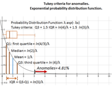
Tukey anomaly criteria for exponential probability distribution function.

Tukey criteria for anomalies.^[4]

The quantile function (inverse cumulative distribution function) for Exp(λ) is

F^{-1}(p;\lambda) = \frac{-\ln(1-p)}{\lambda},\qquad 0 \le p < 1

The quartiles are therefore:

first quartile: ln(4/3)/λ
median: ln(2)/λ
third quartile: ln(4)/λ

And as a consequence the interquartile range is ln(3)/λ.

Kullback–Leibler divergence

The directed Kullback–Leibler divergence of $e^{\lambda}$ ('approximating' distribution) from $e^{\lambda_0}$ ('true' distribution) is given by

\Delta(\lambda_0 || \lambda) = \log(\lambda_0) - \log(\lambda) + \frac{\lambda}{\lambda_0} - 1.

Maximum entropy distribution

Among all continuous probability distributions with support [0, ∞) and mean μ, the exponential distribution with λ = 1/μ has the largest differential entropy. In other words, it is the maximum entropy probability distribution for a random variate X which is greater than or equal to zero and for which E[X] is fixed.^[5]

Distribution of the minimum of exponential random variables

Let X₁, ..., X_n be independent exponentially distributed random variables with rate parameters λ₁, ..., λ_n. Then

\min \left \{X_1,\dotsc,X_n \right \}

is also exponentially distributed, with parameter

\lambda = \lambda_1+\dotsb+\lambda_n

This can be seen by considering the complementary cumulative distribution function:

\begin{align} \Pr \left (\min\{X_1,\dotsc,X_n \} > x \right ) & = \Pr\left(X_1 > x, \dotsc, X_n > x\right) \\ &= \prod_{i=1}^n \Pr(X_i > x) \\ &= \prod_{i=1}^n \exp(-x\lambda_i) = \exp\left(-x\sum_{i=1}^n \lambda_i\right). \end{align}

The index of the variable which achieves the minimum is distributed according to the law

\Pr \left(k|X_{k}=\min\{X_{1},\dotsc ,X_{n}\}\right)={\frac {\lambda _{k}}{\lambda _{1}+\dotsb +\lambda _{n}}}.

Note that

\max\{X_1,\dotsc,X_n\}

is not exponentially distributed.

Parameter estimation

Below, suppose random variable X is exponentially distributed with rate parameter λ, and $x_1, \dotsc, x_n$ are n independent samples from X, with sample mean ${\bar {x}}$ .

Maximum likelihood

The likelihood function for λ, given an independent and identically distributed sample x = (x₁, ..., x_n) drawn from the variable, is:

L(\lambda) = \prod_{i=1}^n \lambda \exp(-\lambda x_i) = \lambda^n \exp \left(-\lambda \sum_{i=1}^n x_i\right)=\lambda^n\exp\left(-\lambda n \overline{x}\right),

where:

\overline{x}={1 \over n}\sum_{i=1}^n x_i

is the sample mean.

The derivative of the likelihood function's logarithm is:

{\frac {{\mathrm {d}}}{{\mathrm {d}}\lambda }}\ln(L(\lambda ))={\frac {{\mathrm {d}}}{{\mathrm {d}}\lambda }}\left(n\ln(\lambda )-\lambda n\overline {x}\right)={\frac {n}{\lambda }}-n\overline {x}\ {\begin{cases}>0,&0<\lambda <{\frac {1}{\overline {x}}},\\[8pt]=0,&\lambda ={\frac {1}{\overline {x}}},\\[8pt]<0,&\lambda >{\frac {1}{\overline {x}}}.\end{cases}}

Consequently, the maximum likelihood estimate for the rate parameter is:

{\widehat {\lambda }}={\frac {1}{\overline {x}}}={\frac {n}{\sum _{i}x_{i}}}

Although this is not an unbiased estimator of $\lambda$ , ${\overline {x}}$ is an unbiased^[6] MLE^[7] estimator of $1/\lambda = \beta,$ where $\beta$ is the scale parameter defined in the 'Alternative parameterization' section above and the distribution mean.

Approximate Minimizer of Expected Squared Error

Assume you have at least three samples. If we seek a minimizer of expected mean squared error (see also: Bias–variance tradeoff) that is similar to the maximum likelihood estimate (i.e. a multiplicative correction to the likelihood estimate) we have:

{\widehat {\lambda }}=\left({\frac {n-2}{n}}\right)\left({\frac {1}{\bar {x}}}\right)={\frac {n-2}{\sum _{i}x_{i}}}

This is derived from the mean and variance of the Inverse-gamma distribution: ${\textstyle {\mbox{Inv-Gamma}}(n,\lambda )}$ .^[8]

Confidence intervals

The 100(1 − α)% confidence interval for the rate parameter of an exponential distribution is given by:^[9]

\frac{2n}{\widehat{\lambda} \chi^2_{1-\frac{\alpha}{2},2n}} < \frac{1}{\lambda} < \frac{2n}{\widehat{\lambda} \chi^2_{\frac{\alpha}{2},2n}}

which is also equal to:

\frac{2n\overline{x}}{\chi^2_{1-\frac{\alpha}{2},2n}} < \frac{1}{\lambda} < \frac{2n\overline{x}}{\chi^2_{\frac{\alpha}{2},2n}}

where $χ 2 p, v$ is the $100(p)$ percentile of the chi squared distribution with v degrees of freedom, n is the number of observations of inter-arrival times in the sample, and x-bar is the sample average. A simple approximation to the exact interval endpoints can be derived using a normal approximation to the $χ 2 p, v$ distribution. This approximation gives the following values for a 95% confidence interval:

\lambda_{low}=\widehat{\lambda} \left (1-\frac{1.96}{\sqrt{n}} \right )

\lambda_{upp}=\widehat{\lambda} \left (1+\frac{1.96}{\sqrt{n}} \right )

This approximation may be acceptable for samples containing at least 15 to 20 elements.^[10]

Bayesian inference

The conjugate prior for the exponential distribution is the gamma distribution (of which the exponential distribution is a special case). The following parameterization of the gamma probability density function is useful:

\mathrm{Gamma}(\lambda; \alpha, \beta) = \frac{\beta^{\alpha}}{\Gamma(\alpha)} \lambda^{\alpha-1} \exp(-\lambda\beta).

The posterior distribution p can then be expressed in terms of the likelihood function defined above and a gamma prior:

\begin{align} p(\lambda) &\propto L(\lambda) \times \mathrm{Gamma}(\lambda; \alpha, \beta) \\ &= \lambda^n \exp\left (-\lambda n\overline{x} \right) \times \frac{\beta^{\alpha}}{\Gamma(\alpha)} \lambda^{\alpha-1} \exp(-\lambda \beta) \\ &\propto \lambda^{(\alpha+n)-1} \exp(-\lambda \left (\beta + n\overline{x} \right)). \end{align}

Now the posterior density p has been specified up to a missing normalizing constant. Since it has the form of a gamma pdf, this can easily be filled in, and one obtains:

p(\lambda) = \mathrm{Gamma}(\lambda; \alpha + n, \beta + n \overline{x}).

Here the hyperparameter α can be interpreted as the number of prior observations, and β as the sum of the prior observations. The posterior mean here is:

\frac{\alpha + n}{\beta + n \overline{x}}.

Generating exponential variates

A conceptually very simple method for generating exponential variates is based on inverse transform sampling: Given a random variate U drawn from the uniform distribution on the unit interval (0, 1), the variate

T = F^{-1}(U)

has an exponential distribution, where F⁻¹ is the quantile function, defined by

F^{-1}(p)=\frac{-\ln(1-p)}{\lambda}.

Moreover, if U is uniform on (0, 1), then so is 1 − U. This means one can generate exponential variates as follows:

T = \frac{-\ln(U)}{\lambda}.

Other methods for generating exponential variates are discussed by Knuth^[11] and Devroye.^[12]

The ziggurat algorithm is a fast method for generating exponential variates.

A fast method for generating a set of ready-ordered exponential variates without using a sorting routine is also available.^[12]

Related distributions

Exponential distribution is closed under scaling by a positive factor. If X ~ Exp(λ) then kX ~ Exp(λ/k).
If X ~ Exp(1/2) then X ∼ χ2
2, i.e. X has a chi-squared distribution with 2 degrees of freedom. Hence:

\exp \left(\lambda \right)={\frac {1}{2\lambda }}\exp \left({\frac {1}{2}}\right)\sim {\frac {1}{2\lambda }}\chi _{2}^{2}\Rightarrow \sum \limits _{i=1}^{n}{\exp \left(\lambda \right)}\sim {\frac {1}{2\lambda }}\chi _{2n}^{2}

If X ~ Exp(λ) and Y ~ Exp(ν) then min(X, Y) ~ Exp(λ + ν).
If X_i ~ Exp(λ) then min{X₁, ..., X_n} ~ Exp(nλ).
The Benktander Weibull distribution reduces to a truncated exponential distribution. If X ~ Exp(λ) then 1+X ~ BenktanderWeibull(λ, 1).
The exponential distribution is a limit of a scaled beta distribution:

\lim_{n \to \infty}n{\rm Beta}(1,n) = {\rm Exp}(1).

If X_i ~ Exp(λ) then the sum X₁ + ... + X_k = $\sum _{i}X_{i}$ ~ Erlang(k, λ) which is just a Gamma(k, λ⁻¹) (in (k, θ) parametrization) or Gamma(k, λ) (in (α,β) parametrization) with an integer shape parameter k.
If X ~ Exp(1) then μ − σ log(X) ~ GEV(μ, σ, 0).
If X ~ Exp(λ) then X ~ Gamma(1, λ⁻¹) (in (k, θ) parametrization) or Gamma(1, λ) (in (α, β) parametrization).
If X ~ Exp(λ) and Y ~ Exp(ν) then λX − νY ~ Laplace(0, 1).
If X, Y ~ Exp(λ) then X − Y ~ Laplace(0, λ⁻¹).
If X ~ Laplace(μ, β⁻¹) then |X − μ| ~ Exp(β).
If X ~ Exp(1) then (logistic distribution):

\mu-\beta\log \left(\tfrac{e^{-X}}{1-e^{-X}}\right) \sim \mathrm{Logistic}(\mu,\beta)

If X, Y ~ Exp(1) then (logistic distribution):

\mu-\beta\log\left(\tfrac{X}{Y}\right) \sim \mathrm{Logistic}(\mu,\beta)

If X ~ Exp(λ) then ke^X ~ Pareto(k, λ).
If X ~ Pareto(1, λ) then log(X) ~ Exp(λ).
Exponential distribution is a special case of type 3 Pearson distribution.
If X ~ Exp(λ) then $\tfrac{e^{-X}}{k} \sim \mathrm{PowerLaw}(k, \lambda)$ (power law)
If X ~ Rayleigh(λ^−1/2) then X²/2 ~ Exp(λ).
If X ~ Exp(λ) then $X \sim \mathrm{Weibull}(\tfrac{1}{\lambda},1)$ (Weibull distribution)
If X_i ~ U(0, 1) then

\lim_{n \to \infty}n \min \left (X_1, \ldots, X_n \right ) \sim \textrm{Exp}(1)

If Y|X ~ Poisson(X) where X ~ Exp(λ⁻¹) then $Y \sim \mathrm{Geometric}(\tfrac{1}{1+\lambda})$ (geometric distribution)
If X ~ Exp(1) and $Y \sim \Gamma(\alpha,\tfrac{\beta}{\alpha})$ then $\sqrt{XY} \sim \mathrm{K}(\alpha,\beta)$ (K-distribution)
The Hoyt distribution can be obtained from Exponential distribution and Arcsine distribution
If X ~ Exp(λ) and Y ~ Erlang(n, λ) then:

\frac{X}{Y} \sim \mathrm{Pareto}(1,n)

If X ~ Exp(λ) and $Y \sim \Gamma(n,\tfrac{1}{\lambda})$ then $\tfrac{X}{Y} \sim \mathrm{Pareto}(1,n)$
If X ~ SkewLogistic(θ), then log(1 + e^−X) ~ Exp(θ).
If X ~ Exp(λ) and Y = μ − β log(Xλ) then Y ∼ Gumbel(μ, β).

Let X ∼ Exp(λ_X) and Y ∼ Exp(λ_Y) be independent. Then $Z = \frac{\lambda_X X}{\lambda_Y Y}$ has probability density function $f_Z(z) = \frac{1}{(z + 1)^2}$ . This can be used to obtain a confidence interval for $\frac{\lambda_X}{\lambda_Y}$ .

Other related distributions:

Hyper-exponential distribution – the distribution whose density is a weighted sum of exponential densities.
Hypoexponential distribution – the distribution of a general sum of exponential random variables.
exGaussian distribution – the sum of an exponential distribution and a normal distribution.

Applications of exponential distribution

Occurrence of events

The exponential distribution occurs naturally when describing the lengths of the inter-arrival times in a homogeneous Poisson process.

The exponential distribution may be viewed as a continuous counterpart of the geometric distribution, which describes the number of Bernoulli trials necessary for a discrete process to change state. In contrast, the exponential distribution describes the time for a continuous process to change state.

In real-world scenarios, the assumption of a constant rate (or probability per unit time) is rarely satisfied. For example, the rate of incoming phone calls differs according to the time of day. But if we focus on a time interval during which the rate is roughly constant, such as from 2 to 4 p.m. during work days, the exponential distribution can be used as a good approximate model for the time until the next phone call arrives. Similar caveats apply to the following examples which yield approximately exponentially distributed variables:

The time until a radioactive particle decays, or the time between clicks of a geiger counter
The time it takes before your next telephone call
The time until default (on payment to company debt holders) in reduced form credit risk modeling

Exponential variables can also be used to model situations where certain events occur with a constant probability per unit length, such as the distance between mutations on a DNA strand, or between roadkills on a given road.

In queuing theory, the service times of agents in a system (e.g. how long it takes for a bank teller etc. to serve a customer) are often modeled as exponentially distributed variables. (The arrival of customers for instance is also modeled by the Poisson distribution if the arrivals are independent and distributed identically.) The length of a process that can be thought of as a sequence of several independent tasks follows the Erlang distribution (which is the distribution of the sum of several independent exponentially distributed variables).

Fitted cumulative exponential distribution to annually maximum 1-day rainfalls using CumFreq^[13]

Reliability theory and reliability engineering also make extensive use of the exponential distribution. Because of the memoryless property of this distribution, it is well-suited to model the constant hazard rate portion of the bathtub curve used in reliability theory. It is also very convenient because it is so easy to add failure rates in a reliability model. The exponential distribution is however not appropriate to model the overall lifetime of organisms or technical devices, because the "failure rates" here are not constant: more failures occur for very young and for very old systems.

In physics, if you observe a gas at a fixed temperature and pressure in a uniform gravitational field, the heights of the various molecules also follow an approximate exponential distribution, known as the Barometric formula. This is a consequence of the entropy property mentioned below.

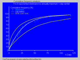
In hydrology, the exponential distribution is used to analyze extreme values of such variables as monthly and annual maximum values of daily rainfall and river discharge volumes.^[14]

The blue picture illustrates an example of fitting the exponential distribution to ranked annually maximum one-day rainfalls showing also the 90% confidence belt based on the binomial distribution. The rainfall data are represented by plotting positions as part of the cumulative frequency analysis.

Prediction

Having observed a sample of n data points from an unknown exponential distribution a common task is to use these samples to make predictions about future data from the same source. A common predictive distribution over future samples is the so-called plug-in distribution, formed by plugging a suitable estimate for the rate parameter λ into the exponential density function. A common choice of estimate is the one provided by the principle of maximum likelihood, and using this yields the predictive density over a future sample x_n+1, conditioned on the observed samples x = (x₁, ..., x_n) given by

p_{\rm ML}(x_{n+1} \mid x_1, \ldots, x_n) = \left( \frac1{\overline{x}} \right) \exp \left( - \frac{x_{n+1}}{\overline{x}} \right)

The Bayesian approach provides a predictive distribution which takes into account the uncertainty of the estimated parameter, although this may depend crucially on the choice of prior.

A predictive distribution free of the issues of choosing priors that arise under the subjective Bayesian approach is

p_{\rm CNML}(x_{n+1} \mid x_1, \ldots, x_n) = \frac{ n^{n+1} \left( \overline{x} \right)^n }{ \left( n \overline{x} + x_{n+1} \right)^{n+1} },

which can be considered as

(1) a frequentist confidence distribution, obtained from the distribution of the pivotal quantity ${x_{n+1}}/{\overline{x}}$ ;^[15]
(2) a profile predictive likelihood, obtained by eliminating the parameter λ from the joint likelihood of x_n+1 and λ by maximization;^[16]
(3) an objective Bayesian predictive posterior distribution, obtained using the non-informative Jeffreys prior 1/λ;
(4) the Conditional Normalized Maximum Likelihood (CNML) predictive distribution, from information theoretic considerations.^[17]

The accuracy of a predictive distribution may be measured using the distance or divergence between the true exponential distribution with rate parameter, λ₀, and the predictive distribution based on the sample x. The Kullback–Leibler divergence is a commonly used, parameterisation free measure of the difference between two distributions. Letting Δ(λ₀||p) denote the Kullback–Leibler divergence between an exponential with rate parameter λ₀ and a predictive distribution p it can be shown that

\begin{align} {\rm E}_{\lambda_0} \left[ \Delta(\lambda_0\mid\mid p_{\rm ML}) \right] &= \psi(n) + \frac{1}{n-1} - \log(n) \\ {\rm E}_{\lambda_0} \left[ \Delta(\lambda_0\mid\mid p_{\rm CNML}) \right] &= \psi(n) + \frac{1}{n} - \log(n) \end{align}

where the expectation is taken with respect to the exponential distribution with rate parameter λ₀ ∈ (0, ∞), and ψ( · ) is the digamma function. It is clear that the CNML predictive distribution is strictly superior to the maximum likelihood plug-in distribution in terms of average Kullback–Leibler divergence for all sample sizes n > 0.

References

↑ https://www.statlect.com/probability-distributions/exponential-distribution
↑ Olkin, Ingram; Gleser, Leon; Derman, Cyrus (1994), Probability Models and Applications (Second ed.), Macmillan, ISBN 0-02-389220-X
↑ David Olive, Chapter 4. Truncated Distributions, "Lemma 4.3", Southern Illinois University, February 18, 2010, p.107.
↑ Template:Ref-missing
↑ Park, Sung Y.; Bera, Anil K. (2009). "Maximum entropy autoregressive conditional heteroskedasticity model" (PDF). Journal of Econometrics. Elsevier: 219–230. Retrieved 2011-06-02.
↑ Richard Arnold Johnson; Dean W. Wichern (2007). Applied Multivariate Statistical Analysis. Pearson Prentice Hall. ISBN 978-0-13-187715-3. Retrieved 10 August 2012.
↑ NIST/SEMATECH e-Handbook of Statistical Methods
↑ Abdulaziz Elfessi and David M. Reineke, "A Bayesian Look at Classical Estimation: The Exponential Distribution", Journal of Statistics Education Volume 9, Number 1 (2001).
↑ Ross, Sheldon M. (2009). Introduction to probability and statistics for engineers and scientists (4th ed.). Associated Press. p. 267. ISBN 978-0-12-370483-2.
↑ Guerriero, V. (2012). "Power Law Distribution: Method of Multi-scale Inferential Statistics". Journal of Modern Mathematics Frontier (JMMF). 1: 21–28.
↑ Donald E. Knuth (1998). The Art of Computer Programming, volume 2: Seminumerical Algorithms, 3rd edn. Boston: Addison–Wesley. ISBN 0-201-89684-2. See section 3.4.1, p. 133.
1 2 Luc Devroye (1986). Non-Uniform Random Variate Generation. New York: Springer-Verlag. ISBN 0-387-96305-7. See chapter IX, section 2, pp. 392–401.
↑ "Cumfreq, a free computer program for cumulative frequency analysis".
↑ Ritzema (ed.), H.P. (1994). Frequency and Regression Analysis (PDF). Chapter 6 in: Drainage Principles and Applications, Publication 16, International Institute for Land Reclamation and Improvement (ILRI), Wageningen, The Netherlands. pp. 175–224. ISBN 90-70754-33-9.
↑ Lawless, J.F., Fredette, M.,"Frequentist predictions intervals and predictive distributions", Biometrika (2005), Vol 92, Issue 3, pp 529–542.
↑ Bjornstad, J.F. (1990). "Predictive Likelihood: A Review". Statist. Sci. 5 (2): 242–254. doi:10.1214/ss/1177012175.
↑ D. F. Schmidt and E. Makalic, "Universal Models for the Exponential Distribution", IEEE Transactions on Information Theory, Volume 55, Number 7, pp. 3087–3090, 2009 doi:10.1109/TIT.2009.2018331

External links

Hazewinkel, Michiel, ed. (2001), "Exponential distribution", Encyclopedia of Mathematics, Springer, ISBN 978-1-55608-010-4
Online calculator of Exponential Distribution

Probability distributions

List

Discrete univariate with finite support	Benford Bernoulli beta-binomial binomial categorical hypergeometric Poisson binomial Rademacher discrete uniform Zipf Zipf–Mandelbrot

Discrete univariate with infinite support	beta negative binomial Borel Conway–Maxwell–Poisson discrete phase-type Delaporte extended negative binomial Gauss–Kuzmin geometric logarithmic negative binomial parabolic fractal Poisson Skellam Yule–Simon zeta

Continuous univariate supported on a bounded interval	arcsine ARGUS Balding–Nichols Bates beta beta rectangular Irwin–Hall Kumaraswamy logit-normal noncentral beta raised cosine reciprocal triangular U-quadratic uniform Wigner semicircle

Continuous univariate supported on a semi-infinite interval	Benini Benktander 1st kind Benktander 2nd kind beta prime Burr chi-squared chi Dagum Davis exponential-logarithmic Erlang exponential F folded normal Flory–Schulz Fréchet gamma gamma/Gompertz generalized inverse Gaussian Gompertz half-logistic half-normal Hotelling's T-squared hyper-Erlang hyperexponential hypoexponential inverse chi-squared scaled inverse chi-squared inverse Gaussian inverse gamma Kolmogorov Lévy log-Cauchy log-Laplace log-logistic log-normal matrix-exponential Maxwell–Boltzmann Maxwell–Jüttner Mittag-Leffler Nakagami noncentral chi-squared Pareto phase-type poly-Weibull Rayleigh relativistic Breit–Wigner Rice shifted Gompertz truncated normal type-2 Gumbel Weibull Discrete Weibull Wilks's lambda

Continuous univariate supported on the whole real line	Cauchy exponential power Fisher's z Gaussian q generalized normal generalized hyperbolic geometric stable Gumbel Holtsmark hyperbolic secant Johnson's S_U Landau Laplace asymmetric Laplace logistic noncentral t normal (Gaussian) normal-inverse Gaussian skew normal slash stable Student's t type-1 Gumbel Tracy–Widom variance-gamma Voigt

Continuous univariate with support whose type varies	generalized extreme value generalized Pareto Tukey lambda q-Gaussian q-exponential q-Weibull shifted log-logistic

Mixed continuous-discrete univariate	rectified Gaussian

Multivariate (joint)	Discrete Ewens multinomial Dirichlet-multinomial negative multinomial Continuous Dirichlet generalized Dirichlet multivariate normal multivariate stable multivariate t normal-inverse-gamma normal-gamma Matrix-valued inverse matrix gamma inverse-Wishart matrix normal matrix t matrix gamma normal-inverse-Wishart normal-Wishart Wishart

Directional	Univariate (circular) directional Circular uniform univariate von Mises wrapped normal wrapped Cauchy wrapped exponential wrapped asymmetric Laplace wrapped Lévy Bivariate (spherical) Kent Bivariate (toroidal) bivariate von Mises Multivariate von Mises–Fisher Bingham

Degenerate and singular	Degenerate Dirac delta function Singular Cantor

Families	Circular compound Poisson elliptical exponential natural exponential location-scale maximum entropy mixture Pearson Tweedie wrapped

Some common univariate probability distributions

Continuous	beta Cauchy chi-squared exponential F gamma Laplace log-normal normal Pareto Student's t uniform Weibull

Discrete	Bernoulli binomial discrete uniform geometric hypergeometric negative binomial Poisson

List of probability distributions

This article is issued from Wikipedia - version of the 11/24/2016. The text is available under the Creative Commons Attribution/Share Alike but additional terms may apply for the media files.

Exponential distribution

Introduction to the exponential distribution

Cumulative distribution function

Examples using the CDF to calculate probability

Exponential distribution in survival analysis

Examples that violate the assumptions of an exponential distribution

Characterization

Probability density function

Cumulative distribution function

Alternative parameterization

Properties

Mean, variance, moments and median

Memorylessness

Quantiles

Kullback–Leibler divergence

Maximum entropy distribution

Distribution of the minimum of exponential random variables

Parameter estimation

Maximum likelihood

Approximate Minimizer of Expected Squared Error

Confidence intervals

Bayesian inference

Generating exponential variates

Related distributions

Applications of exponential distribution

Occurrence of events

Prediction

See also

References

External links