Kuznets curve

Hypothetical Kuznets curve. Empirically observed curves aren't smooth or symmetrical—see reference^[1] for examples of "real" curves.

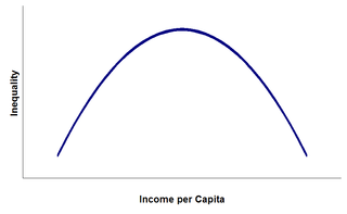
In economics, a Kuznets curve graphs the hypothesis that as an economy develops, market forces first increase and then decrease economic inequality. The hypothesis was first advanced by economist Simon Kuznets in the 1950s and '60s.^[2]

One explanation of such a progression suggests that early in development investment opportunities for those who have money multiply, while an influx of cheap rural labor to the cities holds down wages. Whereas in mature economies, human capital accrual (an estimate of cost that has been incurred but not yet paid) takes the place of physical capital accrual as the main source of growth; and inequality slows growth by lowering education levels because poorer, disadvantaged people lack finance for their education in imperfect credit-markets.

The Kuznets curve implies that as a nation undergoes industrialization – and especially the mechanization of agriculture – the center of the nation’s economy will shift to the cities. As internal migration by farmers looking for better-paying jobs in urban hubs causes a significant rural-urban inequality gap (the owners of firms would be profiting, while laborers from those industries would see their incomes rise at a much slower rate and agricultural workers would possibly see their incomes decrease), rural populations decrease as urban populations increase. Inequality is then expected to decrease when a certain level of average income is reached and the processes of industrialization – democratization and the rise of the welfare state – allow for the trickle-down of the benefits from rapid growth, and increase the per-capita income. Kuznets believed that inequality would follow an inverted “U” shape as it rises and then falls again with the increase of income per-capita.^[3]

Kuznets curve diagrams show an inverted U curve, although variables along the axes are often mixed and matched, with inequality or the Gini coefficient on the Y axis and economic development, time or per-capita incomes on the X axis.

Since 1991 the environmental Kuznets curve (EKC) has become a standard feature in the technical literature of environmental policy,^[4] though its application there has been strongly contested.^[5]

Kuznets ratio

The Kuznets ratio is a measurement of the ratio of income going to the highest-earning households (usually defined by the upper 20%) and the income going to the lowest-earning households,^[6] which is commonly measured by either the lowest 20% or lowest 40% of income. Comparing 20% to 20%, perfect equality is expressed as 1; 20% to 40% changes this value to 0.5.

Kuznets had two similar explanations for this historical phenomenon:

1. workers migrated from agriculture to industry; and
2. rural workers moved to urban jobs.

In both explanations, inequality will decrease after 50% of the shift force switches over to the higher paying sector.^[6]

Criticisms

Critics of the Kuznets curve theory argue that its U-shape comes not from progression in the development of individual countries, but rather from historical differences between countries. For instance, many of the middle income countries used in Kuznets' data set were in Latin America, a region with historically high levels of inequality. When controlling for this variable, the U-shape of the curve tends to disappear (e.g. Deininger and Squire, 1998). Regarding the empirical evidence, based on large panels of countries or time series approaches, Fields (2001) considers the Kuznets hypothesis refuted.^[7]

In accounting for historical changes, David Lempert's work in the early 1980s introduced a time dimension and a political dimension to the curve, showing how population and politics interact with economic inequality over time, leading either to long-term stability or to collapse. This neo-Malthusian model incorporating Kuznets' work, yields a helix model of the relationships over time rather than just a curve.^[8]

The East Asian miracle has been used to criticize the validity of the Kuznets curve theory. The rapid economic growth of eight East Asian countries – Japan, South Korea, Hong Kong, Taiwan, Singapore (Four Asian Tigers), Indonesia, Thailand, and Malaysia – between 1965 and 1990, was called the East Asian miracle (EAM). Manufacturing and export grew quickly and powerfully. Yet simultaneously, life expectancy was found to increase and population levels living in absolute poverty decreased.^[9] This development process was contrary to the Kuznets curve theory. Many studies have been done to identify how the EAM was able to ensure that the benefits of rapid economic growth were distributed broadly among the population, because Kuznets’ theory stated that rapid capital accumulation would lead to an initial increase in inequality.^[10] Joseph Stiglitz argues the East Asian experience of an intensive and successful economic development process along with an immediate decrease in population inequality can be explained by the immediate re-investment of initial benefits into land reform (increasing rural productivity, income, and savings), universal education (providing greater equality and what Stiglitz calls an “intellectual infrastructure” for productivity^[10] ), and industrial policies that distributed income more equally through high and increasing wages and limited the price increases of commodities. These factors increased the average citizen’s ability to consume and invest within the economy, further contributing to economic growth. Stiglitz highlights that the high rates of growth provided the resources to promote equality, which acted as a positive-feedback loop to support the high rates of growth. The EAM defies the Kuznets curve, which insists growth produces inequality, and that inequality is a necessity for overall growth.^[3][10]

Cambridge University Lecturer Gabriel Palma recently found no evidence for a ‘Kuznets curve’ in inequality:

"[T]he statistical evidence for the ‘upwards’ side of the 'Inverted-U' between inequality and income per capita seems to have vanished, as many low and low-middle income countries now have a distribution of income similar to that of most middle-income countries (other than those of Latin America and Southern Africa). That is, half of Sub-Saharan Africa and many countries in Asian, including India, China and Vietnam, now have an income distribution similar to that found in North Africa, the Caribbean and the second-tier NICs. And this level is also similar to that of half of the first-tier NICs, the Mediterranean EU and the Anglophone OECD (excluding the US). As a result, about 80% of the world population now live in countries with a Gini around 40."^[11]

Palma goes on to note that, among middle-income countries, only those in Latin America and Southern Africa live in an inequality league of their own. Instead of a Kuznets curve, he breaks income inequality into deciles which contain 10% of the population relating to income inequality. Palma then shows that there are two distributional trends taking place in inequality within a country:

"One is ‘centrifugal’, and takes place at the two tails of the distribution—leading to an increased diversity across country in the shares appropriated by the top 10 percent and bottom forty percent. The other is ‘centripetal’, and takes place in the middle—leading to a remarkable uniformity across countries in the share of income going to the half of the population located between deciles 5 to 9."^[11]

Therefore, it is the share of the richest 10% of the population that affects the share of the poorest 40% of the population with the middle to upper-middle staying the same across all countries.

Kuznets' own caveats

In a biography about Simon Kuznets' scientific methods, economist Robert Fogel noted Kuznets' own reservations about the "fragility of the data" which underpinned the hypothesis. Fogel notes that most of Kuznets' paper was devoted to explicating the conflicting factors at play. Fogel emphasized Kuznets' opinion that "even if the data turned out to be valid, they pertained to an extremely limited period of time and to exceptional historical experiences." Fogel noted that despite these "repeated warnings", Kuznets' caveats were overlooked, and the Kuznets curve was "raised to the level of law" by other economists.^[12]

Inequality and trade liberalization

Dobson and Ramlogan’s research looked to identify the relationship between inequality and trade liberalization. There have been mixed findings with this idea – some developing countries have experienced greater inequality, less inequality, or no difference at all, due to trade liberalization. Because of this, Dobson and Ramlogan suggest that perhaps trade openness can be related to inequality through a Kuznets curve framework.^[13] A trade liberalization-versus-inequality graph has a measures trade openness along the x-axis and inequality along the y-axis. Dobson and Ramlogan determine trade openness by the ratio of exports and imports (the total trade) and the average tariff rate; inequality is determined by gross primary school enrolment rates, the share of agriculture in total output, the rate of inflation, and cumulative privatization.^[13] By studying data from several Latin American countries that have implemented trade liberalization policies in the past 30 years, the Kuznets curve seems to apply to the relationship between trade liberalization and inequality (measured by the GINI coefficient).^[13] However, many of these nations saw a shift from low-skill labour production to natural resource intensive activities. This shift would not benefit low-skill workers as much. So although their evidence seems to support the Kuznets theory in relation to trade liberalization, Dobson and Ramlogan assert that policies for redistribution must be simultaneously implemented in order to mitigate the initial increase in inequality felt.^[13]

Environmental Kuznets curve

Environmental Kuznets Curve: The application of Kuznets Curve in Environmental Studies.

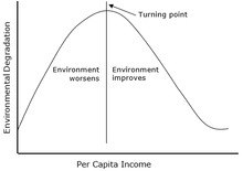
The environmental Kuznets curve is a hypothesized relationship between environmental quality and economic development: various indicators of environmental degradation tend to get worse as modern economic growth occurs until average income reaches a certain point over the course of development.^[14] Although the subject of continuing debate, some evidence supports the claim that environmental health indicators, such as water and air pollution, show the inverted U-shaped curve.^[1] It has been argued that this trend occurs in the level of many of the environmental pollutants, such as sulfur dioxide, nitrogen oxide, lead, DDT, chlorofluorocarbons, sewage, and other chemicals previously released directly into the air or water.

For example, between 1970 and 2006, the United States' inflation-adjusted GDP grew by 195%, the number of cars and trucks in the country more than doubled, and the total number of miles driven increased by 178%. However, during that same time period regulatory changes meant that annual emissions of carbon monoxide fell from 197 million tons to 89 million, nitrogen oxides emissions fell from 27 million tons to 19 million, sulfur dioxide emissions fell from 31 million tons to 15 million, particulate emissions fell by 80%, and lead emissions fell by more than 98%.^[15]

However, there is little evidence that the relationship holds true for other pollutants, for natural resource use or for biodiversity conservation.^[16] For example, energy, land and resource use (sometimes called the "ecological footprint") do not fall with rising income.^[17] While the ratio of energy per real GDP has fallen, total energy use is still rising in most developed countries. Another example is the emission of many greenhouse gases, which is much higher in industrialised countries. In addition, the status of many key "ecosystem services" provided by ecosystems, such as freshwater provision and regulation (Perman, et al., 2003), soil fertility, and fisheries, have continued to decline in developed countries.

In general, Kuznets curves have been found for some environmental health concerns (such as air pollution) but not for others (such as landfills and biodiversity). Advocates of the EKC argue that this does not necessarily invalidate the hypothesis – the scale of the Kuznets curves may differ for different environmental impacts and different regions. If the search for scalar and regional effects can salvage the concept, it may yet be the case that a given area will need more wealth in order to see a decline in environmental pollutants. In contrast, a thermodynamically enlightened economics suggests that outputs of degraded matter and energy are an inescapable consequence of any use of matter and energy (so holds the second law); some of those degraded outputs will be noxious wastes, and whether and how their production is eliminated depends more on regulatory schemes and technologies at use than on income or production levels. In one view, then, the EKC suggests that "the solution to pollution is more economic growth;" in the other, pollution is seen as a regrettable output that should be reduced when the benefits brought by its production are exceeded by the costs it imposes in externalities like health decrements and loss of ecosystem services.

Deforestation may follow a Kuznets curve (cf. forest transition curve). Among countries with a per capita GDP of at least $4,600, net deforestation has ceased to exist.^[18] Yet it has been argued that wealthier countries are able to maintain forests along with high consumption by ‘exporting’ deforestation.^[19]

It has also been suggested that the Kuznets curve applies to both littering and cigarette smoking.^[20]

Criticisms

Critics argue that even the US is still struggling to attain the income level necessary to prioritize certain environmental pollutants such as carbon emissions, which have yet to follow the EKC.^[4] With other pollutants however, like sulfur dioxide, production seems to coincide with a country's economic development and at a certain threshold level of income a mitigation of environmental damage occurs. This could be related rather than causal, because economic growth without institutional reform does not accomplish this environmental improvement. It appears that with GDP growth, government policies are strengthened and populations experience a rise in their demand for improved environmental quality. It may be the case, however, that regulation in relatively wealthy countries simply shifts the production and pollution to less-regulated, poorer countries; if this were true, the total size of the negative externalities of production remains the same or is larger, though in the wealthier country an EKC appears to have been obtained.

This could be a reason why environmental Kuznets curves have been found to be applicable to only certain types of pollutants.^[4] Yandle et al. argue that the EKC has not been found to apply to carbon because most pollutants create localized problems like lead and sulfur, so there is a greater urgency and response to cleaning up such pollutants. As a country develops, the marginal value of cleaning up such pollutants makes a large direct improvement to the quality of citizens' lives. Conversely, reducing carbon dioxide emissions does not have a dramatic impact at a local level, so the impetus to clean them up is only for the altruistic reason of improving the global environment. This becomes a tragedy of the commons where it is most efficient for everyone to pollute and for no one to clean up, and everyone is worse as a result (Hardin, 1968). Thus, even in a country like the US with a high level of income, carbon emissions are not decreasing in accordance with the EKC.^[4]

There seems to be little consensus about whether EKC is formed with regard to CO2 emissions, as CO2 is a global pollutant that has yet to prove its validity within Kuznet's Curve.^[21] Many EKC research papers that touch upon CO2 emissions have been published thus far, with various controversial results regarding the existence of the EKC.^[21] Therefore, the EKC for CO2 remains a matter of further research, and various international measures have been undertaken to address global warming, and so researchers are interested in whether or not some structural changes with regard to CO2 emissions have arisen on account of such measures.^[21] In addition, since CO2 is a global pollutant, its EKC is different depending on countries, and many factors such as whether it is developing or developed with income factors affect the graph.

Arik Levinson points out that researchers disagree about the shape of the curve when longer-term time scales are evaluated. For example, Millimet and Stengos regard the traditional "inverse U" shape as actually being an "N" shape, indicating that pollution increases as a country develops, decreases once the threshold GDP is reached, and then begins increasing as national income continues to increase. While such findings are still being debated, it could prove to be important because it poses the concerning question of whether pollution actually begins to decline for good when an economic threshold is reached or whether the decrease is only in local pollutants and pollution is simply exported to poorer developing countries. Levinson concludes that the environmental Kuznets curve is insufficient to support a pollution policy regardless whether it is laissez-faire or interventionist, although the literature has been used this way by the press.^[22]

Arrow et al. argue pollution-income progression of agrarian communities (clean) to industrial economies (pollution intensive) to service economies (cleaner) would appear to be false if pollution increases again at the end due to higher levels of income and consumption of the population at large.^[23] A difficulty with this model is that it lacks predictive power because it is highly uncertain how the next phase of economic development will be characterized.

Suri and Chapman argue that a net pollution reduction may not actually be occurring on global scales. Wealthy nations have a trend of exporting the activities that create the most pollution, like manufacturing of clothing and furniture, to poorer nations that are still in the process of industrial development (Suri and Chapman, 1998). This could mean that as the world's poor nations develop, they will have nowhere to export their pollution. Thus, this progression of environmental clean up occurring in conjunction with economic growth cannot be replicated indefinitely because there may be nowhere to export waste and pollution intensive processes. However, Gene Grossman and Alan B. Krueger, the authors who initially made the correlation between economic growth, environmental clean-up, and the Kuznets curve, conclude that there is "no evidence that environmental quality deteriorates steadily with economic growth."^[22] And Yandle et al. conclude that "policies that stimulate growth (trade liberalization, economic restructuring, and price reform) should be good for the environment".^[4]

Stern warns "it is very easy to do bad econometrics", and says "the history of the EKC exemplifies what can go wrong". He finds that "Little or no attention has been paid to the statistical properties of the data used such as serial dependence or stochastic trends in time series and few tests of model adequacy have been carried out or presented. However, one of the main purposes of doing econometrics is to test which apparent relationships ... are valid and which are spurious correlations". He states his unequivocal finding: "When we do take such statistics into account and use appropriate techniques we find that the EKC does not exist (Perman and Stern 2003). Instead, we get a more realistic view of the effect of economic growth and technological changes on environmental quality. It seems that most indicators of environmental degradation are monotonically rising in income though the 'income elasticity' is less than one and is not a simple function of income alone. Time related effects reduce environmental impacts in countries at all levels of income. However, in rapidly growing middle income countries the scale effect, which increases pollution and other degradation, overwhelms the time effect. In wealthy countries, growth is slower, and pollution reduction efforts can overcome the scale effect. This is the origin of the apparent EKC effect".^[24]

See also

• Clean growth
• Low-carbon economy
• Bright green environmentalism#Currents

References

Bibliography

• Brenner, Y.S., Hartmut Kaelble, and Mark Thomas (1991): Income Distribution in Historical Perspective. Cambridge University Press.
• Costantini, V.; Monni, S. (2008). "Environment, Human Development and Economic Growth". Ecological Economics. 64 (4): 867–880. doi:10.1016/j.ecolecon.2007.05.011. 
• Dasgupta, S.; Laplante, B.; Wang, H.; Wheeler, D. (2002). "Confronting the Environmental Kuznets Curve". The Journal of Economic Perspectives. 16 (1): 147–168. doi:10.1257/0895330027157. 
• Deacon, R. T.; Norman, C. S. (2006). "Does the Environmental Kuznets Curve Describe How Individual Countries Behave?". Land Economics. 82 (2): 291–315. doi:10.3368/le.82.2.291. 
• Deininger K, Squire L (1998). "New Ways of Looking at Old Issues: Inequality and Growth". Journal of Development Economics. 57 (2): 259–287. doi:10.1016/s0304-3878(98)00099-6. 
• Fields G (2001). Distribution and Development, A New Look at the Developing World. Russel Sage Foundation, New York, and The MIT Press, Cambridge, Massachusetts, and London. 
• Grossman, Gene; Alan B. Krueger (1993). "Environmental Impacts of a North American Free Trade Agreement". In P. Garber. The Mexico-U.S. Free Trade Agreement. Cambridge, Mass.: MIT Press. 
• Harbaugh, B.; Levinson, A.; Wilson, D. (2002). "Reexamining the Empirical Evidence for an Environmental Kuznets Curve". Review of Economics and Statistics. 84 (3). 
• Levinson, Arik (2000). "The Ups and Downs of the Environmental Kuznets Curve" (PDF). Retrieved 10 February 2011. 
• Millennium Ecosystem Assessment (2005). "Ecosystems and Human Wellbeing: Synthesis" (PDF). Island Press. 
• Syed, Munir Khasru; Mohammad, Muaz Jalil (2004). "Revisiting Kuznets Hypothesis: An Analysis with Time Series and Panel Data". Bangladesh Development Studies. 30 (3–4): 89–112. JSTOR 40795695. 
• Palma, JG (2011). "Homogeneous middles vs. heterogeneous tails, and the end of the 'Inverted-U': it's all about the share of the rich". Development and Change. 42: 87–153. doi:10.1111/j.1467-7660.2011.01694.x. 
• Shafik, N., "Economic Development and Environmental Quality: An Econometric Analysis", Oxford Economic Papers, New Series, Vol. 46, Special Issue on Environmental Economics (Oct., 1994), pp. 757–773.
• Tisdell, C. (2001). "Globalisation and sustainability: environmental Kuznets curve and the WTO". Ecological Economics. 39 (2): 185–196. doi:10.1016/s0921-8009(01)00234-8. 
• Van Zanden, J. L. (1995). "Tracing the Beginning of the Kuznets Curve: Western Europe during the Early Modern Period". The Economic History Review. 48 (4): 643–664. doi:10.2307/2598128. 

External links

• John Tierney (20 April 2009). "Use Energy, Get Rich and Save the Planet". New York Times.  Includes links to Further reading:

• Tierney, John (20 April 2009). "The Richer-Is-Greener Curve". New York Times. 
• Tierney, John (22 April 2009). "More on Kuznets curves". New York Times. 

Environmental social science
Fields	Ecological anthropology Ecological economics Environmental anthropology Environmental economics Environmental communication Environmental history Environmental politics Environmental psychology Environmental sociology Human ecology Human geography Political ecology Regional science
Related	Agroecology Anthrozoology Behavioral geography Community studies Demography Design ecological environmental Ecological humanities Economics energy thermo Environmental education ethics law science studies Ethnobiology botany ecology zoology Forestry Industrial ecology Integrated geography Permaculture Rural sociology Science, technology and society science studies Sustainability science studies Systems ecology Urban ecology geography metabolism studies
Applied	Architecture landscape sustainable Ecopsychology Engineering ecological environmental Green criminology Health environmental epidemiology occupational public Management environmental fisheries forest natural resource waste Planning environmental land use regional spatial urban Policy energy environmental
Environment portal Category Concepts Degrees Institutions Journals Research institutes Scholars

References

- 1 2 John Tierney (20 April 2009). "The Richer-Is-Greener Curve". New York Times.
- ↑ Kuznets profile at New School for Social Research: "...his discovery of the inverted U-shaped relation between income inequality and economic growth..."
- 1 2 Galbraith, James (2007). "Global inequality and global macroeconomics". Journal of Policy Modeling. 29 (4): 587–607. doi:10.1016/j.jpolmod.2007.05.008. Retrieved 2 February 2012.
- 1 2 3 4 5 Yandle B, Vijayaraghavan M, Bhattarai M (2000). "The Environmental Kuznets Curve: A Primer". The Property and Environment Research Center. Retrieved 16 June 2008.
- ↑ Roberts, J.T.; Thanos, N.D. (2003), Trouble in Paradise: Globalization and Environmental Crises in Latin America, Routledge: London & New York, p. xiv
- 1 2 Kuznets, Simon. 1955. Economic Growth and Income Inequality. American Economic Review 45 (March): 1–28.