Electric field

Electric field lines emanating from a point positive electric charge suspended over an infinite sheet of conducting material.

Electromagnetism

Electricity Magnetism
Electrostatics Electric charge Static electricity Electric field Conductor Insulator Triboelectricity Electrostatic discharge Induction Coulomb's law Gauss's law Electric flux / potential energy Electric dipole moment Polarization density
Magnetostatics Ampère's law Magnetic field Magnetization Magnetic flux Biot–Savart law Magnetic dipole moment Gauss's law for magnetism
Electrodynamics Lorentz force law Electromagnetic induction Faraday's law Lenz's law Displacement current Magnetic potential Maxwell's equations Electromagnetic field Electromagnetic radiation Maxwell tensor Poynting vector Liénard–Wiechert potential Jefimenko's equations Eddy current London equations Mathematical descriptions of the electromagnetic field
Electrical network Electric current Electric potential Voltage Resistance Ohm's law Series circuit Parallel circuit Direct current Alternating current Charged current Neutral current Electromotive force Capacitance Inductance Impedance Resonant cavities Waveguides
Covariant formulation Electromagnetic tensor (stress–energy tensor) Four-current Electromagnetic four-potential
Scientists Ampère Coulomb Faraday Gauss Heaviside Henry Hertz Lorentz Maxwell Tesla Volta Weber Ørsted

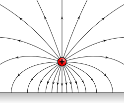
An electric field is a vector field that associates to each point in space the Coulomb force that would be experienced per unit of electric charge, by an infinitesimal test charge at that point.^[1] Electric fields converge and diverge at electric charges and can be induced by time-varying magnetic fields. The electric field combines with the magnetic field to form the electromagnetic field.

Definition

The electric field, $\mathbf {E}$ , at a given point is defined as the (vectorial) force, $\mathbf {F}$ , that would be exerted on a stationary test particle of unit charge by electromagnetic forces (i.e. the Lorentz force). A particle of charge $q$ would be subject to a force $\mathbf{F}=q\cdot\mathbf{E}$ .

Its SI units are newtons per coulomb (N⋅C⁻¹) or, equivalently, volts per metre (V⋅m⁻¹), which in terms of SI base units are kg⋅m⋅s⁻³⋅A⁻¹.

Sources of electric field

Causes and description

Electric fields are caused by electric charges or varying magnetic fields. The former effect is described by Gauss's law, the latter by Faraday's law of induction, which together are enough to define the behavior of the electric field as a function of charge repartition and magnetic field. However, since the magnetic field is described as a function of electric field, the equations of both fields are coupled and together form Maxwell's equations that describe both fields as a function of charges and currents.

In the special case of a steady state (stationary charges and currents), the Maxwell-Faraday inductive effect disappears. The resulting two equations (Gauss's law $\nabla \cdot \mathbf{E} = \frac{\rho}{\varepsilon_0}$ and Faraday's law with no induction term $\nabla \times {\mathbf {E}}=0$ ), taken together, are equivalent to Coulomb's law, written as ${\boldsymbol {E}}({\boldsymbol {r}})={1 \over 4\pi \varepsilon _{0}}\int d{\boldsymbol {r'}}\rho ({\boldsymbol {r'}}){{\boldsymbol {r}}-{\boldsymbol {r'}} \over |{\boldsymbol {r}}-{\boldsymbol {r'}}|^{3}}$ for a charge density ${\mathbf {\rho }}({\mathbf {r}})$ ( $\mathbf {r}$ denotes the position in space). Notice that $\varepsilon _{0}$ , the permittivity of vacuum, must be substituted if charges are considered in non-empty media.

Continuous vs. discrete charge repartition

Main article: Charge density

The equations of electromagnetism are best described in a continuous description. However, charges are sometimes best described as discrete points; for example, some models may describe electrons as point sources where charge density is infinite on an infinitesimal section of space.

A charge $q$ located at ${\mathbf {r_{0}}}$ can be described mathematically as a charge density $\rho ({\mathbf {r}})=q\delta ({\mathbf {r-r_{0}}})$ , where the Dirac delta function (in three dimensions) is used. Conversely, a charge distribution can be approximated by many small point charges.

Superposition principle

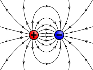
Electric fields satisfy the superposition principle, because Maxwell's equations are linear. As a result, if ${\mathbf {E}}_{1}$ and ${\mathbf {E}}_{2}$ are the electric fields resulting from distribution of charges $\rho _{1}$ and $\rho _{2}$ , a distribution of charges $\rho _{1}+\rho _{2}$ will create an electric field ${\mathbf {E}}_{1}+{\mathbf {E}}_{2}$ ; for instance, Coulomb's law is linear in charge density as well.

This principle is useful to calculate the field created by multiple point charges. If charges $q_{1},q_{2},...,q_{n}$ are stationary in space at ${\mathbf {r}}_{1},{\mathbf {r}}_{2},...{\mathbf {r}}_{n}$ , in the absence of currents, the superposition principle proves that the resulting field is the sum of fields generated by each particle as described by Coulomb's law:

{\mathbf {E}}({\mathbf {r}})=\sum _{{i=1}}^{N}{\mathbf {E}}_{i}({\mathbf {r}})={\frac {1}{4\pi \varepsilon _{0}}}\sum _{{i=1}}^{N}q_{i}{\frac {{\mathbf {r}}-{\mathbf {r}}_{i}}{|{\mathbf {r}}-{\mathbf {r}}_{i}|^{3}}}

Electrostatic fields

Main article: Electrostatics

Illustration of the electric field surrounding a positive (red) and a negative (blue) charge.

Experiment illustrating electric field lines. An electrode connected to an electrostatic induction machine is placed in an oil-filled container. Considering that oil is a dielectric medium, when current is ran through the electrode, the particles arrange themselves so as to show the force lines of the electric field. Performed by Prof. Oliver Zajkov at the Physics Institute at the Ss. Cyril and Methodius University of Skopje, Macedonia.

Electrostatic fields are E-fields which do not change with time, which happens when charges and currents are stationary. In that case, Coulomb's law fully describes the field.

Electric potential

Main article: Conservative vector field § Irrotational vector fields

If a system is static, such that magnetic fields are not time varying, then by Faraday's law, the electric field is curl-free. In this case, one can define an electric potential, that is, a function $\Phi$ such that $\mathbf{E} = -\nabla \Phi$ .^[2] This is analogous to the gravitational potential.

Parallels between electrostatic and gravitational fields

Coulomb's law, which describes the interaction of electric charges:

\mathbf{F}=q\left(\frac{Q}{4\pi\varepsilon_0}\frac{\mathbf{\hat{r}}}{|\mathbf{r}|^2}\right)=q\mathbf{E}

\mathbf{F}=m\left(-GM\frac{\mathbf{\hat{r}}}{|\mathbf{r}|^2}\right)=m\mathbf{g}

(where ${\mathbf {{\hat {r}}}}={\mathbf {{\frac {r}{|r|}}}}$ ).

This suggests similarities between the electric field E and the gravitational field g, or their associated potentials. Mass is sometimes called "gravitational charge" because of that similarity.

Electrostatic and gravitational forces both are central, conservative and obey an inverse-square law.

Uniform fields

A uniform field is one in which the electric field is constant at every point. It can be approximated by placing two conducting plates parallel to each other and maintaining a voltage (potential difference) between them; it is only an approximation because of boundary effects (near the edge of the planes, electric field is distorted because the plane does not continue). Assuming infinite planes, the magnitude of the electric field E is:

E = - \frac{\Delta\phi}{d}

where Δϕ is the potential difference between the plates and d is the distance separating the plates. The negative sign arises as positive charges repel, so a positive charge will experience a force away from the positively charged plate, in the opposite direction to that in which the voltage increases. In micro- and nanoapplications, for instance in relation to semiconductors, a typical magnitude of an electric field is in the order of 7006100000000000000♠10⁶ V⋅m⁻¹, achieved by applying a voltage of the order of 1 volt between conductors spaced 1 µm apart.

Electrodynamic fields

Main article: Electrodynamics

Electrodynamic fields are E-fields which do change with time, for instance when charges are in motion.

The electric field cannot be described independently of the magnetic field in that case. If A is the magnetic vector potential, defined so that $\mathbf{B} = \nabla \times \mathbf{A}$ , one can still define an electric potential $\Phi$ such that:

{\mathbf {E}}=-\nabla \Phi -{\frac {\partial {\mathbf {A}}}{\partial t}}

One can recover Faraday's law of induction by taking the curl of that equation

^[3]

\nabla \times {\mathbf {E}}=-{\frac {\partial (\nabla \times {\mathbf {A}})}{\partial t}}=-{\frac {\partial {\mathbf {B}}}{\partial t}}

which justifies, a posteriori, the previous form for E.

Energy in the electric field

If the magnetic field B is nonzero,

The total energy per unit volume stored by the electromagnetic field is^[4]

u_{{EM}}={\frac {\varepsilon }{2}}|{\mathbf {E}}|^{2}+{\frac {1}{2\mu }}|{\mathbf {B}}|^{2}

where ε is the permittivity of the medium in which the field exists, $\mu$ its magnetic permeability, and E and B are the electric and magnetic field vectors.

As E and B fields are coupled, it would be misleading to split this expression into "electric" and "magnetic" contributions. However, in the steady-state case, the fields are no longer coupled (see Maxwell's equations). It makes sense in that case to compute the electrostatic energy per unit volume:

u_{{ES}}={\frac {1}{2}}\varepsilon |{\mathbf {E}}|^{2}\,,

The total energy U stored in the electric field in a given volume V is therefore

U_{{ES}}={\frac {1}{2}}\varepsilon \int _{{V}}|{\mathbf {E}}|^{2}\,{\mathrm {d}}V\,,

Further extensions

Definitive equation of vector fields

In the presence of matter, it is helpful in electromagnetism to extend the notion of the electric field into three vector fields, rather than just one:^[5]

\mathbf{D}=\varepsilon_0\mathbf{E}+\mathbf{P}\!

where P is the electric polarization – the volume density of electric dipole moments, and D is the electric displacement field. Since E and P are defined separately, this equation can be used to define D. The physical interpretation of D is not as clear as E (effectively the field applied to the material) or P (induced field due to the dipoles in the material), but still serves as a convenient mathematical simplification, since Maxwell's equations can be simplified in terms of free charges and currents.

Constitutive relation

Main article: Constitutive equation

The E and D fields are related by the permittivity of the material, ε.^[6]^[7]

For linear, homogeneous, isotropic materials E and D are proportional and constant throughout the region, there is no position dependence: For inhomogeneous materials, there is a position dependence throughout the material:

\mathbf{D(r)}=\varepsilon\mathbf{E(r)}

For anisotropic materials the E and D fields are not parallel, and so E and D are related by the permittivity tensor (a 2nd order tensor field), in component form:

D_i=\varepsilon_{ij}E_j

For non-linear media, E and D are not proportional. Materials can have varying extents of linearity, homogeneity and isotropy.

References

↑ Richard Feynman (1970). The Feynman Lectures on Physics Vol II. Addison Wesley Longman. ISBN 978-0-201-02115-8.
↑ http://physicspages.com/2011/10/08/curl-potential-in-electrostatics/
↑ Huray, Paul G. (2009). Maxwell's Equations. Wiley-IEEE. p. 205. ISBN 0-470-54276-4.
↑ Introduction to Electrodynamics (3rd Edition), D.J. Griffiths, Pearson Education, Dorling Kindersley, 2007, ISBN 81-7758-293-3
↑ Electromagnetism (2nd Edition), I.S. Grant, W.R. Phillips, Manchester Physics, John Wiley & Sons, 2008, ISBN 978-0-471-92712-9
↑ Electricity and Modern Physics (2nd Edition), G.A.G. Bennet, Edward Arnold (UK), 1974, ISBN 0-7131-2459-8
↑ Electromagnetism (2nd Edition), I.S. Grant, W.R. Phillips, Manchester Physics, John Wiley & Sons, 2008, ISBN 978-0-471-92712-9

External links

Electric field in "Electricity and Magnetism", R Nave – Hyperphysics, Georgia State University
'Gauss's Law' – Chapter 24 of Frank Wolfs's lectures at University of Rochester
'The Electric Field' – Chapter 23 of Frank Wolfs's lectures at University of Rochester
– An applet that shows the electric field of a moving point charge.
Fields – a chapter from an online textbook
Learning by Simulations Interactive simulation of an electric field of up to four point charges
Java simulations of electrostatics in 2-D and 3-D
Interactive Flash simulation picturing the electric field of user-defined or preselected sets of point charges by field vectors, field lines, or equipotential lines. Author: David Chappell

This article is issued from Wikipedia - version of the 11/29/2016. The text is available under the Creative Commons Attribution/Share Alike but additional terms may apply for the media files.