Drag coefficient

Drag coefficients in fluids with Reynolds number approximately 10⁴

In fluid dynamics, the drag coefficient (commonly denoted as: $\scriptstyle C_{{\mathrm d}}\,$ , $\scriptstyle C_{\mathrm {x} }\,$ or $\scriptstyle C_{\mathrm {w} }\,$ ) is a dimensionless quantity that is used to quantify the drag or resistance of an object in a fluid environment, such as air or water. It is used in the drag equation in which a lower drag coefficient indicates the object will have less aerodynamic or hydrodynamic drag. The drag coefficient is always associated with a particular surface area.^[1]

The drag coefficient of any object comprises the effects of the two basic contributors to fluid dynamic drag: skin friction and form drag. The drag coefficient of a lifting airfoil or hydrofoil also includes the effects of lift-induced drag.^[2]^[3] The drag coefficient of a complete structure such as an aircraft also includes the effects of interference drag.^[4]^[5]

Definition

The drag coefficient $c_{{\mathrm d}}\,$ is defined as

c_\mathrm d = \dfrac{ 2F_\mathrm d}{ \rho u^2 A}\,

where:

F_{{\mathrm d}}\,

is the drag force, which is by definition the force component in the direction of the flow velocity,^[6]

\rho \,

is the mass density of the fluid,^[7]

u\,

is the flow speed of the object relative to the fluid,

A\,

is the reference area.

The reference area depends on what type of drag coefficient is being measured. For automobiles and many other objects, the reference area is the projected frontal area of the vehicle. This may not necessarily be the cross sectional area of the vehicle, depending on where the cross section is taken. For example, for a sphere $A=\pi r^{2}\,$ (note this is not the surface area = $\!\ 4\pi r^{2}$ ).

For airfoils, the reference area is the nominal wing area. Since this tends to be large compared to the frontal area, the resulting drag coefficients tend to be low, much lower than for a car with the same drag, frontal area, and speed.

Airships and some bodies of revolution use the volumetric drag coefficient, in which the reference area is the square of the cube root of the airship volume (volume to the two-thirds power). Submerged streamlined bodies use the wetted surface area.

Two objects having the same reference area moving at the same speed through a fluid will experience a drag force proportional to their respective drag coefficients. Coefficients for unstreamlined objects can be 1 or more, for streamlined objects much less.

Background

Flow around a plate, showing stagnation.

Main article: Drag equation

The drag equation

F_d\, =\, \tfrac12\, \rho\, u^2\, c_d\, A

is essentially a statement that the drag force on any object is proportional to the density of the fluid and proportional to the square of the relative flow speed between the object and the fluid.

C_d is not a constant but varies as a function of flow speed, flow direction, object position, object size, fluid density and fluid viscosity. Speed, kinematic viscosity and a characteristic length scale of the object are incorporated into a dimensionless quantity called the Reynolds number $\scriptstyle Re$ . $\scriptstyle C_{{\mathrm d}}\,$ is thus a function of $\scriptstyle Re$ . In a compressible flow, the speed of sound is relevant, and $\scriptstyle C_{{\mathrm d}}\,$ is also a function of Mach number $\scriptstyle Ma$ .

For certain body shapes, the drag coefficient $\scriptstyle C_{{\mathrm d}}\,$ only depends on the Reynolds number $\scriptstyle Re\,$ , Mach number $\scriptstyle Ma\,$ and the direction of the flow. For low Mach number $\scriptstyle Ma$ , the drag coefficient is independent of Mach number. Also, the variation with Reynolds number $\scriptstyle Re\,$ within a practical range of interest is usually small, while for cars at highway speed and aircraft at cruising speed, the incoming flow direction is also more-or-less the same. Therefore, the drag coefficient $\scriptstyle C_{{\mathrm d}}\,$ can often be treated as a constant.^[8]

For a streamlined body to achieve a low drag coefficient, the boundary layer around the body must remain attached to the surface of the body for as long as possible, causing the wake to be narrow. A high form drag results in a broad wake. The boundary layer will transition from laminar to turbulent if Reynolds number of the flow around the body is sufficiently great. Larger velocities, larger objects, and lower viscosities contribute to larger Reynolds numbers.^[9]

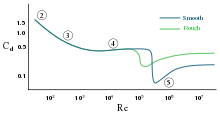
Drag coefficient C_d for a sphere as a function of Reynolds number Re, as obtained from laboratory experiments. The dark line is for a sphere with a smooth surface, while the lighter line is for the case of a rough surface. The numbers along the line indicate several flow regimes and associated changes in the drag coefficient:
•2: attached flow (Stokes flow) and steady separated flow,
•3: separated unsteady flow, having a laminar flow boundary layer upstream of the separation, and producing a vortex street,
•4: separated unsteady flow with a laminar boundary layer at the upstream side, before flow separation, with downstream of the sphere a chaotic turbulent wake,
•5: post-critical separated flow, with a turbulent boundary layer.

For other objects, such as small particles, one can no longer consider that the drag coefficient $\scriptstyle C_{{\mathrm d}}\,$ is constant, but certainly is a function of Reynolds number.^[10]^[11]^[12] At a low Reynolds number, the flow around the object does not transition to turbulent but remains laminar, even up to the point at which it separates from the surface of the object. At very low Reynolds numbers, without flow separation, the drag force $\scriptstyle F_{{\mathrm d}}\,$ is proportional to $\scriptstyle v\,$ instead of $\scriptstyle v^{2}\,$ ; for a sphere this is known as Stokes law. The Reynolds number will be low for small objects, low velocities, and high viscosity fluids.^[9]

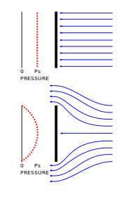
A $\scriptstyle C_{{\mathrm d}}\,$ equal to 1 would be obtained in a case where all of the fluid approaching the object is brought to rest, building up stagnation pressure over the whole front surface. The top figure shows a flat plate with the fluid coming from the right and stopping at the plate. The graph to the left of it shows equal pressure across the surface. In a real flat plate, the fluid must turn around the sides, and full stagnation pressure is found only at the center, dropping off toward the edges as in the lower figure and graph. Only considering the front side, the $\scriptstyle C_{{\mathrm d}}\,$ of a real flat plate would be less than 1; except that there will be suction on the back side: a negative pressure (relative to ambient). The overall $\scriptstyle C_{{\mathrm d}}\,$ of a real square flat plate perpendicular to the flow is often given as 1.17. Flow patterns and therefore $\scriptstyle C_{{\mathrm d}}\,$ for some shapes can change with the Reynolds number and the roughness of the surfaces.

Drag coefficient c_d examples

General

In general, $c_{{\mathrm d}}\,$ is not an absolute constant for a given body shape. It varies with the speed of airflow (or more generally with Reynolds number $Re$ ). A smooth sphere, for example, has a $c_{{\mathrm d}}\,$ that varies from high values for laminar flow to 0.47 for turbulent flow. Although the drag coefficient decreases with increasing $Re$ , the drag force increases.

Shapes
c_d	Item
0.001	laminar flat plate parallel to the flow ( $\!\ Re<10^{6}$ )
0.005	turbulent flat plate parallel to the flow ( $\!\ Re>10^{6}$ )
0.075	Pac-car
0.076	Milan SL (one of the fastest practical velomobiles) ^[13]
0.1	smooth sphere ( $\!\ Re=10^{6}$ )
0.47	smooth sphere ( $\!\ Re=10^{5}$ )
0.15	Schlörwagen 1939 ^[14]
0.18	Mercedes-Benz T80 1939
0.186-0.189	Volkswagen XL1 2014
0.19	General Motors EV1 1996^[15]
0.212	Tatra 77A 1935
0.235	Renault Eolab
0.24	Tesla Model S^[16]
0.24	Toyota Prius (4th Generation)^[17]
0.25	Toyota Prius (3rd Generation)
0.26	BMW i8
0.26	Nissan GT-R (2011-2014)
0.27	Nissan GT-R (2007-2010)
0.28	1969 Dodge Charger Daytona and 1970 Plymouth Superbird
0.28	1986 Opel Omega saloon.^[18]
0.28	Mercedes-Benz CLA-Class Type C 117.^[19]
0.29	Mazda3 (2007) ^[20]
0.295	bullet (not ogive, at subsonic velocity)
0.3	Saab 92 (1949), Audi 100 C3 (1982)
0.31	Maserati Ghibli Sedan (2014) ^[21]
0.324	Ford Focus Mk2/2.5 (2004-2011, Europe)
0.33	BMW E30 3 Series (1984-1993, Germany)
0.35	Maserati Quattroporte V (M139, 2003–2012)
0.36	Citroen CX (1974-1991, France)
0.37	Ford Transit Custom Mk8 (2013, Turkey)
0.48	rough sphere ( $\!\ Re=\!\ 10^{6}$ ), Volkswagen Beetle^[22]^[23]
0.58	Jeep Wrangler TJ (1997-2005)^[24]
0.75	a typical model rocket^[25]
1.0	coffee filter, face-up^[26]
1.0	road bicycle plus cyclist, touring position^[27]
1.0–1.1	skier
1.0–1.3	wires and cables
1.0–1.3	man (upright position)
1.1-1.3	ski jumper^[28]
1.2	Usain Bolt^[29]
1.28	flat plate perpendicular to flow (3D) ^[30]
1.3–1.5	Empire State Building
1.8–2.0	Eiffel Tower
1.98–2.05	flat plate perpendicular to flow (2D)

Aircraft

As noted above, aircraft use their wing area as the reference area when computing $c_{{\mathrm d}}\,$ , while automobiles (and many other objects) use frontal cross sectional area; thus, coefficients are not directly comparable between these classes of vehicles. In the aerospace industry, the drag coefficient is sometimes expressed in drag counts where 1 drag count = 0.0001 of a $C_{d}$ .^[31]

Aircraft^[32]
c_d	Aircraft type
0.021	F-4 Phantom II (subsonic)
0.022	Learjet 24
0.024	Boeing 787^[33]
0.0265	Airbus A380^[34]
0.027	Cessna 172/182
0.027	Cessna 310
0.031	Boeing 747
0.044	F-4 Phantom II (supersonic)
0.048	F-104 Starfighter
0.095	X-15 (Not confirmed)

Blunt and streamlined body flows

Concept

Drag, in the context of fluid dynamics, refers to forces that act on a solid object in the direction of the relative flow velocity (note that the diagram below shows the drag in the opposite direction to the flow). The aerodynamic forces on a body come primarily from differences in pressure and viscous shearing stresses. Thereby, the drag force on a body could be divided into two components, namely frictional drag (viscous drag) and pressure drag (form drag). The net drag force could be decomposed as follows:

Flow across an airfoil showing the relative impact of drag force to the direction of motion of fluid over the body. This drag force gets divided into frictional drag and pressure drag. The same airfoil is considered as a streamlined body if friction drag (viscous drag) dominates pressure drag and is considered a blunt body when pressure drag (form drag) dominates friction drag.

{\begin{aligned}c_{\mathrm {d} }&={\dfrac {2F_{\mathrm {d} }}{\rho v^{2}A}}\ \\&=c_{\mathrm {p} }+c_{\mathrm {f} }\\&=\underbrace {{\dfrac {1}{\rho v^{2}A}}\ \displaystyle \int \limits _{S}\mathrm {d} A\,(p-p_{o})\left({\hat {\mathbf {n} }}\cdot {\hat {\mathbf {i} }}\right)} _{c_{\mathrm {p} }}+\underbrace {{\dfrac {1}{\rho v^{2}A}}\ \displaystyle \int \limits _{S}\mathrm {d} A\,\left({\hat {\mathbf {t} }}\cdot {\hat {\mathbf {i} }}\right)T_{w}} _{c_{\mathrm {f} }}\end{aligned}}

where:

c_{{\mathrm p}}\,

is the pressure drag coefficient,

c_{{\mathrm f}}\,

is the friction drag coefficient,

{\hat {\mathbf {t} }}

= Tangential direction to the surface with area dA,

{\hat {\mathbf {n} }}

= Normal direction to the surface with area dA,

T_{{\mathrm w}}\,

is the shear Stress acting on the surface dA,

p_{{\mathrm o}}\,

is the pressure far away from the surface dA,

p\,

is pressure at surface dA,

{\hat {\mathbf {i} }}

is the unit vector in direction normal to the surface dA, forming a unit vector

\mathrm {d} {\hat {A}}

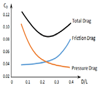
Therefore, when the drag is dominated by a frictional component, the body is called a streamlined body; whereas in the case of dominant pressure drag, the body is called a blunt body. Thus, the shape of the body and the angle of attack determine the type of drag. For example, an airfoil is considered as a body with a small angle of attack by the fluid flowing across it. This means that it has attached boundary layers, which produce much less pressure drag.

Trade-off relationship between pressure drag and friction drag

The wake produced is very small and drag is dominated by the friction component. Therefore, such a body (here an airfoil) is described as streamlined, whereas for bodies with fluid flow at high angles of attack, boundary layer separation takes place. This mainly occurs due to adverse pressure gradients at the top and rear parts of an airfoil.

Due to this, wake formation takes place, which consequently leads to eddy formation and pressure loss due to pressure drag. In such situations, the airfoil is stalled and has higher pressure drag than friction drag. In this case, the body is described as a blunt body.

A streamlined body looks like a fish (Tuna, Oropesa, etc.) or an airfoil with small angle of attack, whereas a blunt body looks like a brick, a cylinder or an airfoil with high angle of attack. For a given frontal area and velocity, a streamlined body will have lower resistance than a blunt body. Cylinders and spheres are taken as blunt bodies because the drag is dominated by the pressure component in the wake region at high Reynolds number.

To reduce this drag, either the flow separation could be reduced or the surface area in contact with the fluid could be reduced (to reduce friction drag). This reduction is necessary in devices like cars, bicycle, etc. to avoid vibration and noise production.

Practical example

The aerodynamic design of cars has evolved from the 1920s to the end of the 20th century. This change in design from a blunt body to a more streamlined body reduced the drag coefficient from about 0.95 to 0.30.

Time history of cars' aerodynamic drag in comparison to change in geometry of streamlined bodies (blunt to streamline).

Notes

↑ McCormick, Barnes W. (1979): Aerodynamics, Aeronautics, and Flight Mechanics. p. 24, John Wiley & Sons, Inc., New York, ISBN 0-471-03032-5
↑ Clancy, L. J.: Aerodynamics. Section 5.18
↑ Abbott, Ira H., and Von Doenhoff, Albert E.: Theory of Wing Sections. Sections 1.2 and 1.3
↑ "NASA's Modern Drag Equation". Wright.nasa.gov. 2010-03-25. Retrieved 2010-12-07.
↑ Clancy, L. J.: Aerodynamics. Section 11.17
↑ See lift force and vortex induced vibration for a possible force components transverse to the flow direction.
↑ Note that for the Earth's atmosphere, the air density can be found using the barometric formula. Air is 1.293 kg/m³ at 0 °C and 1 atmosphere.
↑ Clancy, L. J.: Aerodynamics. Sections 4.15 and 5.4
1 2 Clancy, L. J.: Aerodynamics. Section 4.17
↑ Clift R., Grace J. R., Weber M. E.: Bubbles, drops, and particles. Academic Press NY (1978).
↑ Briens C. L.: Powder Technology. 67, 1991, 87-91.
↑ Haider A., Levenspiel O.: Powder Technology. 58, 1989, 63-70.
↑ "Milan SL". Retrieved 24 March 2015.
↑ "MB-Exotenforum". Retrieved 2012-01-07.
↑ MotorTrend: General Motors EV1 - Driving impression, June 1996
↑ Sherman, Don (2014). "Drag Queens" (PDF). Car and Driver. Retrieved 30 May 2014.
↑ Seabaugh, Christian. "2016 Toyota Prius First Drive Review". MotorTrend. Retrieved 18 November 2015.
↑ http://www.senatorman.de/opel_omega_a.htm. Missing or empty |title= (help)
↑ "Mercedes-Benz CLA-Class Type C 117".
↑ "2007 Mazda 3 - Features & Specs". Edmund's. Retrieved 13 August 2014.
↑ "2014 Maserati Ghibli Sedan - Features & Specs". Edmund's. Retrieved 2 December 2015.
↑ "Technique of the VW Beetle". Maggiolinoweb.it. Retrieved 2009-10-24.
↑ "The Mayfield Homepage - Coefficient of Drag for Selected Vehicles". Mayfco.com. Retrieved 2009-10-24.
↑ "Vehicle Coefficient of Drag List". Retrieved 13 August 2014.
↑ "Terminal Velocity". Goddard Space Center. Retrieved 2012-02-16.
↑ http://www.exo.net/~pauld/activities/flying/TerminalVelocity.html
↑ Wilson, David Gordon (2004): Bicycling Science, 3rd ed.. p. 197, Massachusetts Institute of Technology, Cambridge, ISBN 0-262-23237-5
↑ "Drag Coefficient". Engineeringtoolbox.com. Retrieved 2010-12-07.
↑ Hernandez-Gomez, J J; Marquina, V; Gomez, R W (25 July 2013). "On the performance of Usain Bolt in the 100 m sprint". Eur. J. Phys. IOP. 34 (5): 1227. Bibcode:2013EJPh...34.1227H. doi:10.1088/0143-0807/34/5/1227. Retrieved 23 April 2016.
↑ "Shape Effects on Drag". NASA. Retrieved 2013-03-11.
↑ Basha, W. A. and Ghaly, W. S., "Drag Prediction in Transitional Flow over Airfoils," Journal of Aircraft, Vol. 44, 2007,p. 824–32.
↑ "Ask Us - Drag Coefficient & Lifting Line Theory". Aerospaceweb.org. 2004-07-11. Retrieved 2010-12-07.
↑ "Boeing 787 Dreamliner : Analysis". Lissys.demon.co.uk. 2006-06-21. Retrieved 2010-12-07.
↑ "Airbus A380" (PDF). 2005-05-02. Retrieved 2014-10-06.

References

Clancy, L. J. (1975): Aerodynamics. Pitman Publishing Limited, London, ISBN 0-273-01120-0
Abbott, Ira H., and Von Doenhoff, Albert E. (1959): Theory of Wing Sections. Dover Publications Inc., New York, Standard Book Number 486-60586-8
Hoerner, Dr. Sighard F., Fluid-Dynamic Drag, Hoerner Fluid Dynamics, Bricktown New Jersey, 1965.
Bluff Body: http://www.engineering.uiowa.edu/~me_160/lecture.../Bluff%20Body2.pdf
Drag of Blunt Bodies and Streamlined Bodies: http://www.princeton.edu/~asmits/Bicycle_web/blunt.html
Hucho, W.H., Janssen, L.J., Emmelmann, H.J. 6(1975): The optimization of body details-A method for reducing the aerodynamics drag. SAE 760185.

This article is issued from Wikipedia - version of the 12/1/2016. The text is available under the Creative Commons Attribution/Share Alike but additional terms may apply for the media files.