Double pendulum

A double pendulum consists of two pendulums attached end to end.

In physics and mathematics, in the area of dynamical systems, a double pendulum is a pendulum with another pendulum attached to its end, and is a simple physical system that exhibits rich dynamic behavior with a strong sensitivity to initial conditions.^[1] The motion of a double pendulum is governed by a set of coupled ordinary differential equations and is chaotic.

Analysis and interpretation

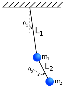
Several variants of the double pendulum may be considered; the two limbs may be of equal or unequal lengths and masses, they may be simple pendulums or compound pendulums (also called complex pendulums) and the motion may be in three dimensions or restricted to the vertical plane. In the following analysis, the limbs are taken to be identical compound pendulums of length $\ell$ and mass $m$ , and the motion is restricted to two dimensions.

Double compound pendulum

In a compound pendulum, the mass is distributed along its length. If the mass is evenly distributed, then the center of mass of each limb is at its midpoint, and the limb has a moment of inertia of $\textstyle I={\frac {1}{12}}m\ell ^{2}$ about that point.

It is convenient to use the angles between each limb and the vertical as the generalized coordinates defining the configuration of the system. These angles are denoted θ₁ and θ₂. The position of the center of mass of each rod may be written in terms of these two coordinates. If the origin of the Cartesian coordinate system is taken to be at the point of suspension of the first pendulum, then the center of mass of this pendulum is at:

x_{1}={\frac {\ell }{2}}\sin \theta _{1},

y_{1}=-{\frac {\ell }{2}}\cos \theta _{1}

and the center of mass of the second pendulum is at

x_{2}=\ell \left(\sin \theta _{1}+{\frac {1}{2}}\sin \theta _{2}\right),

y_{2}=-\ell \left(\cos \theta _{1}+{\frac {1}{2}}\cos \theta _{2}\right).

This is enough information to write out the Lagrangian.

Lagrangian

The Lagrangian is

{\begin{aligned}L&=\mathrm {Kinetic~Energy} -\mathrm {Potential~Energy} \\&={\frac {1}{2}}m\left(v_{1}^{2}+v_{2}^{2}\right)+{\frac {1}{2}}I\left({{\dot {\theta }}_{1}}^{2}+{{\dot {\theta }}_{2}}^{2}\right)-mg\left(y_{1}+y_{2}\right)\\&={\frac {1}{2}}m\left({{\dot {x}}_{1}}^{2}+{{\dot {y}}_{1}}^{2}+{{\dot {x}}_{2}}^{2}+{{\dot {y}}_{2}}^{2}\right)+{\frac {1}{2}}I\left({{\dot {\theta }}_{1}}^{2}+{{\dot {\theta }}_{2}}^{2}\right)-mg\left(y_{1}+y_{2}\right)\end{aligned}}

The first term is the linear kinetic energy of the center of mass of the bodies and the second term is the rotational kinetic energy around the center of mass of each rod. The last term is the potential energy of the bodies in a uniform gravitational field. The dot-notation indicates the time derivative of the variable in question.

Substituting the coordinates above and rearranging the equation gives

L={\frac {1}{6}}m\ell ^{2}\left[{{\dot {\theta }}_{2}}^{2}+4{{\dot {\theta }}_{1}}^{2}+3{{\dot {\theta }}_{1}}{{\dot {\theta }}_{2}}\cos(\theta _{1}-\theta _{2})\right]+{\frac {1}{2}}mg\ell \left(3\cos \theta _{1}+\cos \theta _{2}\right).

Trajectories of a double pendulum

Long exposure of double pendulum exhibiting chaotic motion (tracked with an LED)

There is only one conserved quantity (the energy), and no conserved momenta. The two momenta may be written as

p_{\theta _{1}}={\frac {\partial L}{\partial {{\dot {\theta }}_{1}}}}={\frac {1}{6}}m\ell ^{2}\left[8{{\dot {\theta }}_{1}}+3{{\dot {\theta }}_{2}}\cos(\theta _{1}-\theta _{2})\right]

and

p_{\theta _{2}}={\frac {\partial L}{\partial {{\dot {\theta }}_{2}}}}={\frac {1}{6}}m\ell ^{2}\left[2{{\dot {\theta }}_{2}}+3{{\dot {\theta }}_{1}}\cos(\theta _{1}-\theta _{2})\right].

These expressions may be inverted to get

{{\dot {\theta }}_{1}}={\frac {6}{m\ell ^{2}}}{\frac {2p_{\theta _{1}}-3\cos(\theta _{1}-\theta _{2})p_{\theta _{2}}}{16-9\cos ^{2}(\theta _{1}-\theta _{2})}}

and

{{\dot {\theta }}_{2}}={\frac {6}{m\ell ^{2}}}{\frac {8p_{\theta _{2}}-3\cos(\theta _{1}-\theta _{2})p_{\theta _{1}}}{16-9\cos ^{2}(\theta _{1}-\theta _{2})}}.

The remaining equations of motion are written as

{{\dot {p}}_{\theta _{1}}}={\frac {\partial L}{\partial \theta _{1}}}=-{\frac {1}{2}}m\ell ^{2}\left[{{\dot {\theta }}_{1}}{{\dot {\theta }}_{2}}\sin(\theta _{1}-\theta _{2})+3{\frac {g}{\ell }}\sin \theta _{1}\right]

and

{{\dot {p}}_{\theta _{2}}}={\frac {\partial L}{\partial \theta _{2}}}=-{\frac {1}{2}}m\ell ^{2}\left[-{{\dot {\theta }}_{1}}{{\dot {\theta }}_{2}}\sin(\theta _{1}-\theta _{2})+{\frac {g}{\ell }}\sin \theta _{2}\right].

These last four equations are explicit formulae for the time evolution of the system given its current state. It is not possible to go further and integrate these equations analytically, to get formulae for θ₁ and θ₂ as functions of time. It is however possible to perform this integration numerically using the Runge Kutta method or similar techniques.

Chaotic motion

Graph of the time for the pendulum to flip over as a function of initial conditions

The double pendulum undergoes chaotic motion, and shows a sensitive dependence on initial conditions. The image to the right shows the amount of elapsed time before the pendulum "flips over," as a function of initial conditions. Here, the initial value of θ₁ ranges along the x-direction, from −3 to 3. The initial value θ₂ ranges along the y-direction, from −3 to 3. (Presumably, this exposition is describing a stationary release with kinetic terms at zero.) The colour of each pixel indicates whether either pendulum flips within $10{\sqrt {\ell /g}}$ (green), within $100{\sqrt {\ell /g}}$ (red), $1000{\sqrt {\ell /g}}$ (purple) or $10000{\sqrt {\ell /g}}$ (blue). Initial conditions that don't lead to a flip within $10000{\sqrt {\ell /g}}$ are plotted white.

The boundary of the central white region is defined in part by energy conservation with the following curve:

3\cos \theta _{1}+\cos \theta _{2}=2.\,

Within the region defined by this curve, that is if

3\cos \theta _{1}+\cos \theta _{2}>2,\,

then it is energetically impossible for either pendulum to flip. Outside this region, the pendulum can flip, but it is a complex question to determine when it will flip. Similar behavior is observed for a double pendulum composed of two point masses rather than two rods with distributed mass.^[2]

The lack of a natural excitation frequency has led to the use of double pendulum systems in seismic resistance designs in buildings, where the building itself is the primary inverted pendulum, and a secondary mass is connected to complete the double pendulum.

Notes

↑ Levien RB and Tan SM. Double Pendulum: An experiment in chaos.American Journal of Physics 1993; 61 (11): 1038
↑ Alex Small, Sample Final Project: One Signature of Chaos in the Double Pendulum, (2013). A report produced as an example for students. Includes a derivation of the equations of motion, and a comparison between the double pendulum with 2 point masses and the double pendulum with 2 rods.

References

Meirovitch, Leonard (1986). Elements of Vibration Analysis (2nd ed.). McGraw-Hill Science/Engineering/Math. ISBN 0-07-041342-8.
Eric W. Weisstein, Double pendulum (2005), ScienceWorld (contains details of the complicated equations involved) and "Double Pendulum" by Rob Morris, Wolfram Demonstrations Project, 2007 (animations of those equations).
Peter Lynch, Double Pendulum, (2001). (Java applet simulation.)
Northwestern University, Double Pendulum, (Java applet simulation.)
Theoretical High-Energy Astrophysics Group at UBC, Double pendulum, (2005).

External links

Animations and explanations of a double pendulum and a physical double pendulum (two square plates) by Mike Wheatland (Univ. Sydney)
Interactive Javascript simulation of a double pendulum
Double pendulum physics simulation from www.myphysicslab.com using open source JavaScript code
Simulation, equations and explanation of Rott's pendulum
Comparison videos of a double pendulum with the same initial starting conditions on YouTube
Double Pendulum Simulator - An open source simulator written in C++ using the Qt toolkit.
Online Java simulator of the Imaginary exhibition.
Free Simulator Android App Two double pendulums side by side - watch divergence of close initial conditions / see periodic orbits.

Chaos theory

Chaos theory	Anosov diffeomorphism Bifurcation theory Butterfly effect Chaos theory in organizational development Complexity Control of chaos Dynamical system Edge of chaos Fractal Predictability Quantum chaos Santa Fe Institute Synchronization of chaos Unintended consequences

Chaotic maps (list)	Arnold tongue Arnold's cat map Baker's map Complex quadratic map Complex squaring map Coupled map lattice Double pendulum Double scroll attractor Duffing equation Duffing map Dyadic transformation Dynamical billiards outer Exponential map Gauss map Gingerbreadman map Hénon map Horseshoe map Ikeda map Interval exchange map Kaplan–Yorke map Logistic map Lorenz system Multiscroll attractor Rabinovich–Fabrikant equations Rössler attractor Standard map Swinging Atwood's machine Tent map Tinkerbell map Van der Pol oscillator Zaslavskii map

Chaos systems	Bouncing ball dynamics Chua's circuit Economic bubble Tilt-A-Whirl

Chaos theorists	Michael Berry Leon O. Chua Mitchell Feigenbaum Martin Gutzwiller Brosl Hasslacher Michel Hénon Edward Norton Lorenz Aleksandr Lyapunov Benoît Mandelbrot Henri Poincaré Otto Rössler David Ruelle Oleksandr Mykolaiovych Sharkovsky Floris Takens James A. Yorke

This article is issued from Wikipedia - version of the 11/29/2016. The text is available under the Creative Commons Attribution/Share Alike but additional terms may apply for the media files.