Distributed minimum spanning tree

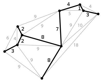
Example of a MST: The minimum spanning tree of a planar graph. Each edge is labeled with its weight, which here is roughly proportional to its length.

The distributed minimum spanning tree (MST) problem involves the construction of a minimum spanning tree by a distributed algorithm, in a network where nodes communicate by message passing. It is radically different from the classical sequential problem, although the most basic approach resembles Borůvka's algorithm. One important application of this problem is to find a tree that can be used for broadcasting. In particular, if the cost for a message to pass through an edge in a graph is significant, a MST can minimize the total cost for a source process to communicate with all the other processes in the network.

The problem was first suggested and solved in $O(V \log V)$ time in 1983 by Gallager et al.,^[1] where $V$ is the number of vertices in the graph. Later, the solution was improved to $O(V)$ ^[2] and finally^[3]^[4] $O(\sqrt V \log^* V + D)$ where D is the network, or graph diameter. A lower bound on the time complexity of the solution has been eventually shown to be^[5] $\Omega\left({\frac{\sqrt V}{\log V}}\right).$

Overview

The input graph $G(V,E)$ is considered to be a network, where vertices $V$ are independent computing nodes and edges $E$ are communication links. Links are weighted as in the classical problem.

At the beginning of the algorithm, nodes know only the weights of the links which are connected to them. (It is possible to consider models in which they know more, for example their neighbors' links.)

As the output of the algorithm, every node knows which of its links belong to the Minimum Spanning Tree and which do not.

MST in message-passing model

The message-passing model is one of the most commonly used models in distributed computing. In this model, each process is modeled as a node of a graph. The communication channel between two processes is an edge of the graph.

Two commonly used algorithms for the classical minimum spanning tree problem are Prim’s algorithm and Kruskal’s algorithm. However, it is difficult to apply these two algorithms in the distributed message-passing model. The main challenges are:

Both Prim’s algorithm and Kruskal’s algorithm require processing one node or vertex at a time, making it difficult to make them run in parallel. (For example, Kruskal's algorithm processes edges in turn, deciding whether to include the edge in the MST based on whether it would form a cycle with all previously chosen edges.)
Both Prim’s algorithm and Kruskal’s algorithm require processes to know the state of the whole graph, which is very difficult to discover in the message-passing model.

Due to these difficulties, new techniques were needed for distributed MST algorithms in the message-passing model. Some bear similarities to Borůvka's algorithm for the classical MST problem.

GHS algorithm

The GHS algorithm of Gallager, Humblet and Spira is one of the best-known algorithms in distributed computing theory. This algorithm can construct the MST in asynchronous Message-passing model.

Preconditions^[1]

The algorithm should run on a connected undirected graph.
The graph should have distinct finite weights assigned to each edge. (This assumption can be removed by breaking ties between edge weights in a consistent way.)
Each node initially knows the weight for each edge incident to that node.
Initially, each node is in a quiescent state and it either spontaneously awakens or is awakened by receipt of any message from another node.
Messages can be transmitted independently in both directions on an edge and arrive after an unpredictable but finite delay, without error.
Each edge delivers messages in FIFO order.

Properties of MST

Define fragment of a MST T to be a sub-tree of T, that is, a connected set of nodes and edges of T. There are two properties of MSTs:

Given a fragment of a MST T, let e be a minimum-weight outgoing edge of the fragment. Then joining e and its adjacent non-fragment node to the fragment yields another fragment of an MST.^[1]
If all the edges of a connected graph have different weights, then the MST of the graph is unique.^[1]

These two properties form the basis for proving correctness of the GHS algorithm. In general, the GHS algorithm is a bottom-up algorithm in the sense that it starts by letting each individual node be a fragment and joining fragments in a certain way to form new fragments. This process of joining fragments repeats until there is only one fragment left and property 1 and 2 imply the resulting fragment is a MST.

Description of the algorithm

The GHS algorithm assigns a level to each fragment, which is a non-decreasing integer with initial value 0. Each non-zero level fragment has an ID, which is the ID of the core edge in the fragment, which is selected when the fragment is constructed. During the execution of the algorithm, each node can classify each of its incident edges into three categories:^[1]^[6]

Branch edges are those that have already been determined to be part of the MST.
Rejected edges are those that have already been determined not to be part of the MST.
Basic edges are neither branch edges nor rejected edges.

For level-0 fragments, each awakened node will do the following:

Choose its minimum-weight incident edge and marks that edge as a branch edge.
Send a message via the branch edge to notify the node on the other side.
Wait for a message from the other end of the edge.

The edge chosen by both nodes it connects becomes the core with level 1.

For a non-zero level fragment, an execution of the algorithm can be separated into three stages in each level:

Broadcast

The two nodes adjacent to the core broadcast messages to the rest of the nodes in the fragment. The messages are sent via the branch edge but not via the core. Each broadcast message contains the ID and level of the fragment. At the end of this stage, each node has received the new fragment ID and level.

Convergecast

In this stage, all nodes in the fragment cooperate to find the minimum weight outgoing edge of the fragment. Outgoing edges are edges connecting to other fragments. The messages sent in this stage are in the opposite direction of the broadcast stage. Initialized by all the leaves (the nodes that have only one branch edge), a message is sent through the branch edge. The message contains the minimum weight of the incident outgoing edge it found (or infinity if no such edge was found). The way to find the minimum outgoing edge will be discussed later. For each non-leaf node, (let the number of its branch edges be n) after receiving n-1 convergecast messages, it will pick the minimum weight from the messages and compare it to the weights of its incident outgoing edges. The smallest weight will be sent toward the branch it received the broadcast from.

Change core

After the completion of the previous stage, the two nodes connected by the core can inform each other of the best edges they received. Then they can identify the minimum outgoing edge from the entire fragment. A message will be sent from the core to the minimum outgoing edge via a path of branch edges. Finally, a message will be sent out via the chosen outgoing edge to request to combine the two fragments that the edge connects. Depending on the levels of those two fragments, one of two combined operations are performed to form a new fragment (details discussed below).

How to find minimum weight incident outgoing edge?

As discussed above, every node needs to find its minimum weight outgoing incident edge after the receipt of a broadcast message from the core. If node n receives a broadcast, it will pick its minimum weight basic edge and send a message to the node n’ on the other side with its fragment’s ID and level. Then, node n’ will decide whether the edge is an outgoing edge and send back a message to notify node n of the result. The decision is made according to the following:
Case 1: Fragment_ID(n) = Fragment_ID(n’).
Then, node n and n’ belongs to same fragment (so the edge is not outgoing).
Case 2: Fragment_ID(n) != Fragment_ID(n’) and Level(n) <= Level(n’).
Then, node n and n’ belongs to the different fragments (so the edge is outgoing).
Case 3: Fragment_ID(n) != Fragment_ID(n’) and Level(n) > Level(n’).
We cannot make any conclusion. The reason is the two nodes may belong to the same fragment already but node n’ has not discovered this fact yet due to the delay of a broadcast message. In this case, the algorithm lets node n’ postpone the response until its level becomes higher than or equal to the level it received from node n.

How to combine two fragments?

Let F and F’ be the two fragments that need to be combined. There are two ways to do this:^[1]^[6]

Merge: This operation occurs if both F and F’ share a common minimum weight outgoing edge, and Level(F) = Level(F’). The level of the combined fragment will be Level(F) + 1.
Absorb: This operation occurs if Level(F) < Level(F’). The combined fragment will have the same level as F’.

Furthermore, when an "Absorb" operation occurs, F must be in the stage of changing the core while F’ can be in arbitrary stage. Therefore, "Absorb" operations may be done differently depending on the state of F’. Let e be the edge that F and F’ want to combine with and let n and n’ be the two nodes connected by e in F and F’, respectively. There are two cases to consider:
Case 1: Node n’ has received broadcast message but it has not sent a convergecast message back to the core.
In this case, fragment F can simply join the broadcast process of F’. Specifically, we image F and F’ have already combined to form a new fragment F’’, so we want to find the minimum weight outgoing edge of F’’. In order to do that, node n’ can initiate a broadcast to F to update the fragment ID of each node in F and collect minimum weight outgoing edge in F.
Case 2: Node n’ has already sent a convergecast message back to the core.
Before node n’ sent a convergecast message, it must have picked a minimum weight outgoing edge. As we discussed above, n’ does that by choosing its minimum weight basic edge, sending a test message to the other side of the chosen edge, and waiting for the response. Suppose e’ is the chosen edge, we can conclude the following:

e’ != e
weight(e’) < weight(e)

The second statement follows if the first one holds. For the first statement, suppose n’ chose the edge e and sent a test message to n via edge e. Then, node n will delay the response (according to case 3 of "How to find minimum weight incident outgoing edge?"). Then, it is impossible that n’ has already sent its convergecast message. By 1 and 2, we can conclude it is safe to absorb F into F' since e’ is still the minimum outgoing edge to report after F is absorbed.

Maximum number of levels

As mentioned above, fragments are combined by either "Merge" or "Absorb" operation. "Absorb" operation doesn't change the maximum level among all fragments. "Merge" operation may increase the maximum level by 1. In the worst case, all fragments are combined with "Merge" operations, so the number of fragments decreases by half in each level. Therefore, the maximum number of levels is $O(\log V)$ , where V is the number of nodes.

Progress property

This algorithm has a nice property that the lowest level fragments will not be blocked, although some operations in non-lowest level fragments may be blocked. This property implies the algorithm will eventually terminate with a minimum spanning tree.

Approximation algorithms

An $O(\log n)$ -approximation algorithm was developed by Maleq Khan and Gopal Pandurangan.^[7] This algorithm runs in $O(D+L\log n)$ time, where $L$ is the local shortest path diameter^[7] of the graph.

References

1 2 3 4 5 6 Robert G. Gallager, Pierre A. Humblet, and P. M. Spira, “A distributed algorithm for minimum-weight spanning trees,” ACM Transactions on Programming Languages and Systems, vol. 5, no. 1, pp. 66–77, January 1983.
↑ Baruch Awerbuch. “Optimal Distributed Algorithms for Minimum Weight Spanning Tree, Counting, Leader Election, and Related Problems,” Proceedings of the 19th ACM Symposium on Theory of Computing (STOC), New York City, New York, May 1987.
↑ Juan Garay, Shay Kutten and David Peleg, “A Sub-Linear Time Distributed Algorithm for Minimum-Weight Spanning Trees (Extended Abstract),” Proceedings of the IEEE Symposium on Foundations of Computer Science (FOCS), 1993.
↑ Shay Kutten and David Peleg, “Fast Distributed Construction of Smallk-Dominating Sets and Applications,” Journal of Algorithms, Volume 28, Issue 1, July 1998, Pages 40-66.
↑ David Peleg and Vitaly Rubinovich “A near tight lower bound on the time complexity of Distributed Minimum Spanning Tree Construction,“ SIAM Journal on Computing, 2000, and IEEE Symposium on Foundations of Computer Science (FOCS), 1999.
1 2 Nancy A. Lynch. Distributed Algorithms. Morgan Kaufmann, 1996.
1 2 Maleq Khan and Gopal Pandurangan. “A Fast Distributed Approximation Algorithm for Minimum Spanning Trees,” Distributed Computing, vol. 20, no. 6, pp. 391–402, Apr. 2008.

This article is issued from Wikipedia - version of the 2/17/2015. The text is available under the Creative Commons Attribution/Share Alike but additional terms may apply for the media files.