Discrete wavelet transform

An example of the 2D discrete wavelet transform that is used in JPEG2000. The original image is high-pass filtered, yielding the three large images, each describing local changes in brightness (details) in the original image. It is then low-pass filtered and downscaled, yielding an approximation image; this image is high-pass filtered to produce the three smaller detail images, and low-pass filtered to produce the final approximation image in the upper-left.

In numerical analysis and functional analysis, a discrete wavelet transform (DWT) is any wavelet transform for which the wavelets are discretely sampled. As with other wavelet transforms, a key advantage it has over Fourier transforms is temporal resolution: it captures both frequency and location information (location in time).

Examples

Haar wavelets

Main article: Haar wavelet

The first DWT was invented by Hungarian mathematician Alfréd Haar. For an input represented by a list of $2^{n}$ numbers, the Haar wavelet transform may be considered to pair up input values, storing the difference and passing the sum. This process is repeated recursively, pairing up the sums to provide the next scale, which leads to $2^{n}-1$ differences and a final sum.

Daubechies wavelets

Main article: Daubechies wavelet

The most commonly used set of discrete wavelet transforms was formulated by the Belgian mathematician Ingrid Daubechies in 1988. This formulation is based on the use of recurrence relations to generate progressively finer discrete samplings of an implicit mother wavelet function; each resolution is twice that of the previous scale. In her seminal paper, Daubechies derives a family of wavelets, the first of which is the Haar wavelet. Interest in this field has exploded since then, and many variations of Daubechies' original wavelets were developed.^[1]

The dual-tree complex wavelet transform (DℂWT)

The dual-tree complex wavelet transform (ℂWT) is a relatively recent enhancement to the discrete wavelet transform (DWT), with important additional properties: It is nearly shift invariant and directionally selective in two and higher dimensions. It achieves this with a redundancy factor of only $2^{d}$ substantially lower than the undecimated DWT. The multidimensional (M-D) dual-tree ℂWT is nonseparable but is based on a computationally efficient, separable filter bank (FB).^[2]

Others

Other forms of discrete wavelet transform include the non- or undecimated wavelet transform (where downsampling is omitted), the Newland transform (where an orthonormal basis of wavelets is formed from appropriately constructed top-hat filters in frequency space). Wavelet packet transforms are also related to the discrete wavelet transform. Complex wavelet transform is another form.

Properties

The Haar DWT illustrates the desirable properties of wavelets in general. First, it can be performed in $O(n)$ operations; second, it captures not only a notion of the frequency content of the input, by examining it at different scales, but also temporal content, i.e. the times at which these frequencies occur. Combined, these two properties make the Fast wavelet transform (FWT) an alternative to the conventional fast Fourier transform (FFT).

Time issues

Due to the rate-change operators in the filter bank, the discrete WT is not time-invariant but actually very sensitive to the alignment of the signal in time. To address the time-varying problem of wavelet transforms, Mallat and Zhong proposed a new algorithm for wavelet representation of a signal, which is invariant to time shifts.^[3] According to this algorithm, which is called a TI-DWT, only the scale parameter is sampled along the dyadic sequence 2^j (j∈Z) and the wavelet transform is calculated for each point in time.^[4]^[5]

Applications

The discrete wavelet transform has a huge number of applications in science, engineering, mathematics and computer science. Most notably, it is used for signal coding, to represent a discrete signal in a more redundant form, often as a preconditioning for data compression. Practical applications can also be found in signal processing of accelerations for gait analysis,^[6] in digital communications and many others.^[7] ^[8]^[9]

It is shown that discrete wavelet transform (discrete in scale and shift, and continuous in time) is successfully implemented as analog filter bank in biomedical signal processing for design of low-power pacemakers and also in ultra-wideband (UWB) wireless communications.^[10]

Comparison with Fourier transform

Definition

One level of the transform

The DWT of a signal $x$ is calculated by passing it through a series of filters. First the samples are passed through a low pass filter with impulse response $g$ resulting in a convolution of the two:

y[n]=(x*g)[n]=\sum \limits _{{k=-\infty }}^{\infty }{x[k]g[n-k]}

The signal is also decomposed simultaneously using a high-pass filter $h$ . The outputs giving the detail coefficients (from the high-pass filter) and approximation coefficients (from the low-pass). It is important that the two filters are related to each other and they are known as a quadrature mirror filter.

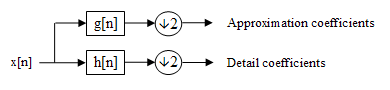
However, since half the frequencies of the signal have now been removed, half the samples can be discarded according to Nyquist’s rule. The filter output of the low-pass filter $g$ in the diagram above is then subsampled by 2 and further processed by passing it again through a new low- pass filter $g$ and a high- pass filter $h$ with half the cut-off frequency of the previous one,i.e.:

y_{\mathrm {low} }[n]=\sum \limits _{k=-\infty }^{\infty }{x[k]g[2n-k]}

y_{\mathrm {high} }[n]=\sum \limits _{k=-\infty }^{\infty }{x[k]h[2n-k]}

This decomposition has halved the time resolution since only half of each filter output characterises the signal. However, each output has half the frequency band of the input, so the frequency resolution has been doubled.

With the subsampling operator $\downarrow$

(y \downarrow k)[n] = y[k n]

the above summation can be written more concisely.

y_{\mathrm{low}} = (x*g)\downarrow 2

y_{\mathrm{high}} = (x*h)\downarrow 2

However computing a complete convolution $x*g$ with subsequent downsampling would waste computation time.

The Lifting scheme is an optimization where these two computations are interleaved.

Cascading and filter banks

This decomposition is repeated to further increase the frequency resolution and the approximation coefficients decomposed with high and low pass filters and then down-sampled. This is represented as a binary tree with nodes representing a sub-space with a different time-frequency localisation. The tree is known as a filter bank.

At each level in the above diagram the signal is decomposed into low and high frequencies. Due to the decomposition process the input signal must be a multiple of $2^{n}$ where $n$ is the number of levels.

For example a signal with 32 samples, frequency range 0 to $f_{n}$ and 3 levels of decomposition, 4 output scales are produced:

Level	Frequencies	Samples
3	$0$ to ${{f_n}}/8$	4
3	${{f_n}}/8$ to ${{f_n}}/4$	4
2	${{f_n}}/4$ to ${{f_n}}/2$	8
1	${{f_n}}/2$ to $f_{n}$	16

Relationship to the Mother Wavelet

The filterbank implementation of wavelets can be interpreted as computing the wavelet coefficients of a discrete set of child wavelets for a given mother wavelet $\psi(t)$ . In the case of the discrete wavelet transform, the mother wavelet is shifted and scaled by powers of two

$\psi_{j,k}(t)= \frac{1}{\sqrt{2^j}} \psi \left( \frac{t - k 2^j}{2^j} \right)$

where $j$ is the scale parameter and $k$ is the shift parameter, both which are integers.

Recall that the wavelet coefficient $\gamma$ of a signal $x(t)$ is the projection of $x(t)$ onto a wavelet, and let $x(t)$ be a signal of length $2^N$ . In the case of a child wavelet in the discrete family above,

$\gamma_{jk} = \int_{-\infty}^{\infty} x(t) \frac{1}{\sqrt{2^j}} \psi \left( \frac{t - k 2^j}{2^j} \right) dt$

Now fix $j$ at a particular scale, so that $\gamma_{jk}$ is a function of $k$ only. In light of the above equation, $\gamma_{jk}$ can be viewed as a convolution of $x(t)$ with a dilated, reflected, and normalized version of the mother wavelet, $h(t) = \frac{1}{\sqrt{2^j}} \psi \left( \frac{-t}{2^j} \right)$ , sampled at the points $1, 2^j, 2^{2j}, ..., 2^{N}$ . But this is precisely what the detail coefficients give at level $j$ of the discrete wavelet transform. Therefore, for an appropriate choice of $h[n]$ and $g[n]$ , the detail coefficients of the filter bank correspond exactly to a wavelet coefficient of a discrete set of child wavelets for a given mother wavelet $\psi(t)$ .

As an example, consider the discrete Haar wavelet, whose mother wavelet is $\psi = [1, -1]$ . Then the dilated, reflected, and normalized version of this wavelet is $h[n] = \frac{1}{\sqrt{2}} [-1, 1]$ , which is, indeed, the highpass decomposition filter for the discrete Haar wavelet transform.

Time complexity

The filterbank implementation of the Discrete Wavelet Transform takes only O(N) in certain cases, as compared to O(N log N) for the fast Fourier transform.

Note that if $g[n]$ and $h[n]$ are both a constant length (i.e. their length is independent of N), then $x * h$ and $x * g$ each take O(N) time. The wavelet filterbank does each of these two O(N) convolutions, then splits the signal into two branches of size N/2. But it only recursively splits the upper branch convolved with $g[n]$ (as contrasted with the FFT, which recursively splits both the upper branch and the lower branch). This leads to the following recurrence relation

T(N)=2N+T\left({\frac {N}{2}}\right)

which leads to an O(N) time for the entire operation, as can be shown by a geometric series expansion of the above relation.

As an example, the discrete Haar wavelet transform is linear, since in that case $h[n]$ and $g[n]$ are constant length 2.

h[n] = \left[\frac{-\sqrt{2}}{2}, \frac{\sqrt{2}}{2}\right] g[n] = \left[\frac{\sqrt{2}}{2}, \frac{\sqrt{2}}{2}\right]

Other transforms

Code example

In its simplest form, the DWT is remarkably easy to compute.

The Haar wavelet in Java:

public static int[] discreteHaarWaveletTransform(int[] input) {
    // This function assumes that input.length=2^n, n>1
    int[] output = new int[input.length];

    for (int length = input.length >> 1; ; length >>= 1) {
        // length = input.length / 2^n, WITH n INCREASING to log_2(input.length)
        for (int i = 0; i < length; ++i) {
            int sum = input[i * 2] + input[i * 2 + 1];
            int difference = input[i * 2] - input[i * 2 + 1];
            output[i] = sum;
            output[length + i] = difference;
        }
        if (length == 1) {
            return output;
        }

        //Swap arrays to do next iteration
        System.arraycopy(output, 0, input, 0, length << 1);
    }
}

Complete Java code for a 1-D and 2-D DWT using Haar, Daubechies, Coiflet, and Legendre wavelets is available from the open source project: JWave. Furthermore, a fast lifting implementation of the discrete biorthogonal CDF 9/7 wavelet transform in C, used in the JPEG 2000 image compression standard can be found here (archived 5 March 2012).

Example of above code

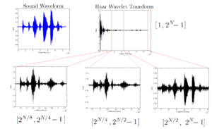
An example of computing the discrete Haar wavelet coefficients for a sound signal of someone saying "I Love Wavelets." The original waveform is shown in blue in the upper left, and the wavelet coefficients are shown in black in the upper right. Along the bottom is shown three zoomed-in regions of the wavelet coefficients for different ranges.

This figure shows an example of applying the above code to compute the Haar wavelet coefficients on a sound waveform. This example highlights two key properties of the wavelet transform:

Natural signals often have some degree of smoothness, which makes them sparse in the wavelet domain. There are far fewer significant components in the wavelet domain in this example than there are in the time domain, and most of the significant components are towards the coarser coefficients on the left. Hence, natural signals are compressible in the wavelet domain.
The wavelet transform is a multiresolution, bandpass representation of a signal. This can be seen directly from the filterbank definition of the discrete wavelet transform given in this article. For a signal of length $2^N$ , the coefficients in the range $[2^{\frac{N}{j+1}}, 2^{\frac{N}{j}}-1]$ represent a version of the original signal which is in the pass-band $\left[ \frac{\pi}{2^j}, \frac{\pi}{2^{j-1}} \right]$ . This is why zooming in on these ranges of the wavelet coefficients looks so similar in structure to the original signal. Ranges which are closer to the left (larger $j$ in the above notation), are coarser representations of the signal, while ranges to the right represent finer details.

Notes

References

↑ Akansu, Ali N.; Haddad, Richard A. (1992), Multiresolution signal decomposition: transforms, subbands, and wavelets, Boston, MA: Academic Press, ISBN 978-0-12-047141-6
↑ Selesnick, I.W.; Baraniuk, R.G.; Kingsbury, N.C., 2005, The dual-tree complex wavelet transform
↑ S. Mallat, A Wavelet Tour of Signal Processing, 2nd ed. San Diego, CA: Academic, 1999.
↑ S. G. Mallat and S. Zhong, “Characterization of signals from multiscale edges,” IEEE Trans. Pattern Anal. Mach. Intell., vol. 14, no. 7, pp. 710– 732, Jul. 1992.
↑ Ince, Kiranyaz, Gabbouj, 2009, A generic and robust system for automated patient-specific classification of ECG signals
↑ "Novel method for stride length estimation with body area network accelerometers", IEEE BioWireless 2011, pp. 79–82
↑ A.N. Akansu and M.J.T. Smith, Subband and Wavelet Transforms: Design and Applications, Kluwer Academic Publishers, 1995.
↑ A.N. Akansu and M.J. Medley, Wavelet, Subband and Block Transforms in Communications and Multimedia, Kluwer Academic Publishers, 1999.
↑ A.N. Akansu, P. Duhamel, X. Lin and M. de Courville Orthogonal Transmultiplexers in Communication: A Review, IEEE Trans. On Signal Processing, Special Issue on Theory and Applications of Filter Banks and Wavelets. Vol. 46, No.4, pp. 979–995, April, 1998.
↑ A.N. Akansu, W.A. Serdijn, and I.W. Selesnick, Wavelet Transforms in Signal Processing: A Review of Emerging Applications, Physical Communication, Elsevier, vol. 3, issue 1, pp. 1–18, March 2010.

External links

Stanford's WaveLab in matlab
libdwt, a cross-platform DWT library written in C

This article is issued from Wikipedia - version of the 11/27/2016. The text is available under the Creative Commons Attribution/Share Alike but additional terms may apply for the media files.