Different types of boundary conditions in fluid dynamics

For more details on this topic, see Computational fluid dynamics.

The most integral part of any Computational fluid dynamics (CFD) problem is the definition of its boundary conditions. Therefore, it is required that the user understands and uses the boundary conditions correctly, wisely and effectively and also understands its role in the numerical algorithm. If the boundary conditions are not specified correctly, then the solution might result in blunders and if they are not utilized wisely, then the problem solving time may increase manifold. Transient problems require one more thing i.e., initial conditions where initial values of flow variables are specified at nodes in the flow domain.^[1] Various types of boundary conditions are used in CFD for different conditions and purposes and are discussed as follows.

Inlet boundary conditions

Showing inlet flow velocity in a pipe

In inlet boundary conditions, the distribution of all flow variables needs to be specified at inlet boundaries mainly flow velocity.^[1] This type of boundary conditions is common and specified mostly where inlet flow velocity is known.

Outlet boundary condition

Showing outlet flow velocity in a pipe

In outlet boundary conditions, the distribution of all flow variables needs to be specified at outlet boundaries mainly flow velocity. This can be thought as a conjunction to inlet boundary condition. This type of boundary conditions is common and specified mostly where outlet velocity is known.^[1] The flow attains a fully developed state where no change occurs in the flow direction when the outlet is selected far away from the geometrical disturbances. In such region, an outlet could be outlined and the gradient of all variables could be equated to zero in the flow direction except pressure.

Wall boundary condition

Showing wall boundary condition

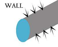
The most common boundary that comes upon in the confined fluid flow problems is the Wall. This is also commonly known as no-slip boundary condition and this is the appropriate conditions for velocity components at the wall. The normal component could be set to zero straightaway while the tangential component is set to the velocity of the wall.^[1]

$V_{\textrm {normal}}=0$
$V_{\textrm {tangential}}=V_{\textrm {wall}}$

Heat transfer through the wall can be specified or if the walls are considered adiabatic, then heat transfer across the wall is set to zero.

$Q_{\textrm {AdiabaticWalls}}=0$

Constant pressure boundary conditions

Showing constant pressure boundary condition

This type of boundary condition is used where boundary values of pressure are known and the exact details of the flow distribution are unknown. This includes pressure inlet and outlet conditions mainly. Typical examples that utilize this boundary condition include buoyancy driven flows, internal flows with multiple outlets, free surface flows and external flows around objects.^[1] An example can be of flow outlet into atmosphere where pressure is atmospheric.

Axisymmetric boundary conditions

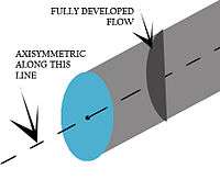
Showing axisymmetric boundary condition

In this boundary condition, the model is axisymmetric with respect to the main axis such that at a particular r = R, all θs and each z = Z-slice, each flow variable has the same value.^[2] A good example is the flow in a circular pipe where the flow and pipe axes coincide.

$V_{r}(R,\theta ,Z)=Constant$ $(r=R,\theta ,Z)$

Symmetric boundary condition

Showing symmetric boundary condition

In this boundary condition, it is assumed that on the two sides of the boundary, same physical processes exist.^[3] All the variables have same value and gradients at the same distance from the boundary. It acts as a mirror that reflects all the flow distribution to the other side.^[4] The conditions at symmetric boundary are

No flow across boundary
No scalar flux across boundary

A good example is of a pipe flow with a symmetric obstacle in the flow. The obstacle divides the upper flow and lower flow as mirrored flow.

Periodic or cyclic boundary condition

A quarter showing cyclic boundary condition

Periodic or Cyclic boundary condition arises from a different type of symmetry in a problem. If a component has a repeated pattern in flow distribution more than twice, thus violating the mirror image requirements required for symmetric boundary condition. A good example would be swept vane pump (Fig.),^[5] where the marked area is repeated four times in r-theta coordinates. The cyclic-symmetric areas should have the same flow variables and distribution and should satisfy that in every Z-slice.^[1]

Notes

1 2 3 4 5 6 Henk Kaarle Versteeg; Weeratunge Malalasekera (1995). An Introduction to Computational Fluid Dynamics: The Finite Volume Method. Longman Scientific & Technical. pp. 192–206. ISBN 0-582-21884-5.
↑ "cyclic symmetric BCs". Retrieved 2015-08-09.
↑ "cyclic symmetric BCs". Retrieved 2013-10-10.
↑ "Symmetric boundary condition".
↑ "cyclic symmetric BCs". Retrieved 2013-10-10.

References

Versteeg (1995). "Chapter 9". An Introduction to Computational Fluid Dynamics The Finite Volume Method, 2/e. Longman Scientific & Technical. pp. 192–206. ISBN 0-582-21884-5.
"Symmetric boundary condition".
"cyclic symmetric BCs". Retrieved 2013-10-10.

This article is issued from Wikipedia - version of the 10/8/2016. The text is available under the Creative Commons Attribution/Share Alike but additional terms may apply for the media files.