De Rham curve
In mathematics, a de Rham curve is a certain type of fractal curve named in honor of Georges de Rham.
The Cantor function, Cesàro curve, Minkowski's question mark function, the Lévy C curve, the blancmange curve and the Koch curve are all special cases of the general de Rham curve.
Construction
Consider some metric space  (generally
  2 with the usual euclidean distance), and a pair of contracting maps on M:


By the Banach fixed point theorem, these have fixed points  and
and  respectively. Let x be a real number in the interval
 ![[0,1]](../I/m/ccfcd347d0bf65dc77afe01a3306a96b.png) , having binary expansion
, having binary expansion

where each  is 0 or 1. Consider the map
defined by

where  denotes function composition. It can be shown that each
  will map the common basin of attraction of
  and
and  to a single point
  in
in  . The collection of points , parameterized by a single real parameter x, is known as the de Rham curve.
Continuity condition
When the fixed points are paired such that

then it may be shown that the resulting curve is a continuous function of x. When the curve is continuous, it is not in general differentiable.
In the remaining of this page, we will assume the curves are continuous.
Properties
De Rham curves are by construction self-similar, since
 for
for ![x \in [0, 1/2]](../I/m/e47b16ecb86430902e708becd487cd20.png) and
and  for
for ![x \in [1/2, 1].](../I/m/6c978d71aeffc7b270a08c11b7767b35.png)
The self-symmetries of all of the de Rham curves are given by the monoid that describes the symmetries of the infinite binary tree or Cantor set. This so-called period-doubling monoid is a subset of the modular group.
The image of the curve, i.e. the set of points ![\{p(x), x \in [0,1]\}](../I/m/643c79e1ebd55df337c3a300b6646c9f.png) , can be obtained by an Iterated function system using the set of contraction mappings
, can be obtained by an Iterated function system using the set of contraction mappings  . But the result of an iterated function system with two contraction mappings is a de Rham curve if and only if the contraction mappings satisfy the continuity condition.
Classification and examples
Cesàro curves


Cesàro curves (or Cesàro-Faber curves) are De Rham curves generated by affine transformations conserving orientation, with fixed points  and
and  .
.
Because of these constraints, Cesàro curves are uniquely determined by a complex number  such that
  and
and  .
.
The contraction mappings and are then defined as complex functions in the complex plane by:

For the value of  , the resulting curve is the Lévy C curve.
Koch–Peano curves
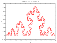

In a similar way, we can define the Koch–Peano family of curves as the set of De Rham curves generated by affine transformations reversing orientation, with fixed points and .
These mappings are expressed in the complex plane as a function of  , the complex conjugate of
  :
:

The name of the family comes from its two most famous members. The Koch curve is obtained by setting:
while the Peano curve corresponds to:

General affine maps
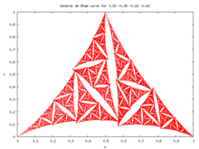
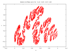
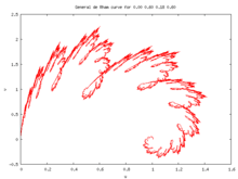

The Cesàro-Faber and Peano-Koch curves are both special cases of the general case of a pair of affine linear transformations on the complex plane. By fixing one endpoint of the curve at 0 and the other at one, the general case is obtained by iterating on the two transforms
and
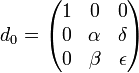
Being affine transforms, these transforms act on a point  of the 2-D plane by acting on the vector

The midpoint of the curve can be seen to be located at  ; the other four parameters may be varied to create a large variety of curves.
The blancmange curve of parameter  can be obtained by setting
 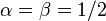 ,
,  and
and  . That is:
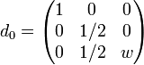
and
Since the blancmange curve of parameter  is the parabola of equation
  , this illustrate the fact that in some occasion, de Rham curves can be smooth.
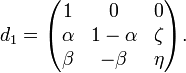
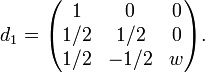
Minkowski's question mark function
Minkowski's question mark function is generated by the pair of maps
and
Generalizations
It is easy to generalize the definition by using more than two contraction mappings. If one uses n mappings, then the n-ary decomposition of x has to be used instead of the binary expansion of real numbers. The continuity condition has to be generalized in:
 , for
, for 
Such a generalization allows, for example, to produce the Sierpiński arrowhead curve (whose image is the Sierpiński triangle), by using the contraction mappings of an iterated function system that produces the Sierpiński triangle.
See also
References
- Georges de Rham, On Some Curves Defined by Functional Equations (1957), reprinted in Classics on Fractals, ed. Gerald A. Edgar (Addison-Wesley, 1993), pp. 285–298.
- Georges de Rham, Sur quelques courbes definies par des equations fonctionnelles. Univ. e Politec. Torino. Rend. Sem. Mat., 1957, 16, 101 –113
- Linas Vepstas, A Gallery of de Rham curves, (2006).
- Linas Vepstas, Symmetries of Period-Doubling Maps, (2006). (A general exploration of the modular group symmetry in fractal curves.)