Data parallelism
Data parallelism is a form of parallelization across multiple processors in parallel computing environments. It focuses on distributing the data across different nodes, which operate on the data in parallel. It can be applied on regular data structures like arrays and matrices by working on each element in parallel. It contrasts to task parallelism as another form of parallelism.
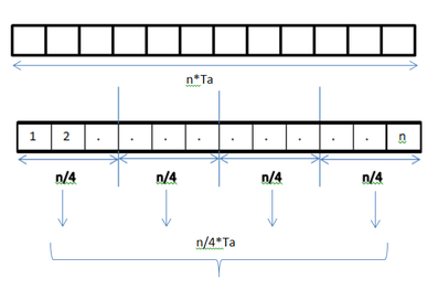
A data parallel job on an array of 'n' elements can be divided equally among all the processors. Let us assume we want to sum all the elements of the given array and the time for a single addition operation is Ta time units. In the case of sequential execution, the time taken by the process will be n*Ta time units as it sums up all the elements of an array. On the other hand, if we execute this job as a data parallel job on 4 processors the time taken would reduce to (n/4)*Ta + Merging overhead time units. Parallel execution results in a speedup of 4 over sequential execution. One important thing to note is that the locality of data references plays an important part in evaluating the performance of a data parallel programming model. Locality of data depends on the memory accesses performed by the program as well as the size of the cache.
History
Exploitation of the concept of Data Parallelism started in 1960s with the development of Solomon machine. Solomon machine, also called a vector processor wanted to expedite the math performance by working on a large data array(operating on multiple data in consecutive time steps). Concurrency of data was also exploited by operating on multiple data points at the same time using a single instruction. These generation of processors were called Array Processors.[1] Today, data parallelism is best exemplified in graphics processing units(GPUs) which use both the techniques of operating on multiple data points in space and time using a single instruction.
Description
In a multiprocessor system executing a single set of instructions (SIMD), data parallelism is achieved when each processor performs the same task on different pieces of distributed data. In some situations, a single execution thread controls operations on all pieces of data. In others, different threads control the operation, but they execute the same code.
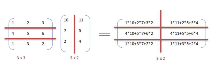
For instance, consider matrix multiplication and addition in a sequential manner as discussed in the example.
Example
Below is the sequential pseudo-code for multiplication and addition of two matrices where the result is stored in the matrix C. The pseudo-code for multiplication calculates the dot product of two matrices A, B and stores the result into the output matrix C.
If the following programs were executed sequentially, the time taken to calculate the result would be of the (assuming row lengths and column lengths of both matrices are n) and for multiplication and addition respectively.


//Matrix Multiplication
for(i=0; i<row_length_A; i++)
{
        for (k=0; k<column_length_B; k++)
        {
                sum = 0;
                for (j=0; j<column_length_A; j++)
                {
                        sum += A[i][j]*B[j][k];
                }
                C[i][k]=sum;
        }
}
//Array addition
for(i=0;i<n;i++) {
    c[i]=a[i]+b[i];
    }
We can exploit data parallelism in the preceding codes to execute it faster as the arithmetic is loop independent. Parallelization of the matrix multiplication code is achieved by using OpenMP. An OpenMP directive, "omp parallel for" instructs the compiler to execute the code in the for loop in parallel. For multiplication, we can divide matrix A and B into blocks along rows and columns respectively. This allows us to calculate every element in matrix C individually thereby making the task parallel. For example: A[m x n] dot B [n x k] can be finished in instead of when executed in parallel using m*k processors.

//Matrix multiplication in parallel
#pragma omp parallel for schedule(dynamic,1) collapse(2)
for(i=0; i<row_length_A; i++){
        for (k=0; k<column_length_B; k++){
                sum = 0;
                for (j=0; j<column_length_A; j++){
                        sum += A[i][j]*B[j][k];
                }
                C[i][k]=sum;
        }
}
It can be observed from the example that a lot of processors will be required as the matrix sizes keep on increasing. Keeping the execution time low is the priority but as the matrix size increases, we are faced with other constraints like complexity of such a system and its associated costs. Therefore, constraining the number of processors in the system, we can still apply the same principle and divide the data into bigger chunks to calculate the product of two matrices.[2]
For addition of arrays in a data parallel implementation, let’s assume a more modest system with two Central Processing Units (CPU) A and B, CPU A could add all elements from the top half of the arrays, while CPU B could add all elements from the bottom half of the arrays. Since the two processors work in parallel, the job of performing array addition would take one half the time of performing the same operation in serial using one CPU alone.
The program expressed in pseudocode below—which applies some arbitrary operation, foo, on every element in the array d—illustrates data parallelism:[nb 1]
if CPU = "a"
    lower_limit := 1
    upper_limit := round(d.length/2)
else if CPU = "b"
    lower_limit := round(d.length/2) + 1
    upper_limit := d.length

for i from lower_limit to upper_limit by 1
    foo(d[i])
In an SPMD system executed on 2 processor system, both CPUs will execute the code.
Data parallelism emphasizes the distributed (parallel) nature of the data, as opposed to the processing (task parallelism). Most real programs fall somewhere on a continuum between task parallelism and data parallelism.
Steps to parallelization
The process of parallelizing a sequential program can be broken down into four discrete steps.[3]
| Type | Description |
|---|---|
| Decomposition | The program is broken down into tasks, the smallest exploitable unit of concurrence. |
| Assignment | Tasks are assigned to processes. |
| Orchestration | Data access, communication, and synchronization of processes. |
| Mapping | Processes are bound to processors. |
Data parallelism vs. task parallelism
| Data Parallelism | Task Parallelism |
| Same operations are performed on different subsets of same data structure. | Different operations are performed on the same or different data in parallel to fully utilize the resources. |
| Synchronous computation | Asynchronous computation |
| Speedup is more as there is only one execution thread operating on all sets of data. | Speedup is less as each processor will execute a different thread or process on the same or different set of data. |
| Amount of parallelization is proportional to the input data size. | Amount of parallelization is proportional to the number of functions to be performed. |
| Designed for optimum load balance on multi processor system. | Load balancing depends on the availability of the hardware and scheduling algorithms like static and dynamic scheduling. |
Data Parallelism vs. Model Parallelism[4]
| Data Parallelism | Model Parallelism |
| Same model is used for every thread but the data given to each of them is divided and shared. | Same data is used for every thread, and model is split among threads. |
| It is fast for small networks but very slow for large networks since large amounts of data needs to be transferred between processors all at once. | It is slow for small networks and fast for large networks. |
| Data parallelism is ideally used in array and matrix computations and convolutional neural networks | Model parallelism finds its applications in deep learning |
Mixed data and task parallelism[5]
Data and task parallelism, can be simultaneously implemented by combining them together for the same application. This is called Mixed data and task parallelism. Mixed parallelism requires sophisticated scheduling algorithms and software support. It is the best kind of parallelism when communication is slow and number of processors is large.
Mixed data and task parallelism has many applications. It is particularly used in the following applications:
- Mixed data and task parallelism finds applications in the global climate modeling. Large data parallel computations are performed by creating grids of data representing earth’s atmosphere and oceans and task parallelism is employed for simulating the function and model of the physical processes.
- In timing based circuit simulation. The data is divided among different sub-circuits and parallelism is achieved with orchestration from the tasks.
Data parallel programming environments
A variety of data parallel programming environments are available today, most widely used of which are:
- Message Passing Interface: It is a cross-platform message passing programming interface for parallel computers. It defines the semantics of library functions to allow users to write portable message passing programs in C, C++ and Fortran.
- Open Multi Processing[6] (Open MP): It’s an Application Programming Interface (API) which supports shared memory programming models on multiple platforms of multiprocessor systems .
- CUDA: CUDA is another parallel computing API platform designed by Nvidia to allow a software engineer to utilize GPU’s computational units.
Applications
Data Parallelism finds its applications in a variety of fields ranging from physics, chemistry, biology, material sciences to signal processing. Sciences imply data parallelism for simulating models like molecular dynamics,[7] sequence analysis of genome data [8] and other physical phenomenon. Driving forces in signal processing for data parallelism are video encoding, image and graphics processing, wireless communications [9] to name a few.
See also
- Active message
- Instruction level parallelism
- Scalable parallelism
- Thread level parallelism
- Parallel programming model
Notes
- ↑ Some input data (e.g. when
d.lengthevaluates to 1 androundrounds towards zero [this is just an example, there are no requirements on what type of rounding is used]) will lead tolower_limitbeing greater thanupper_limit, it's assumed that the loop will exit immediately (i.e. zero iterations will occur) when this happens.
References
- ↑ "SIMD/Vector/GPU" (PDF). Retrieved 2016-09-07.
- ↑ Barney, Blaise. "Introduction to Parallel Computing". computing.llnl.gov. Retrieved 2016-09-07.
- ↑ Solihin, Yan (2016). Fundamentals of Parallel Architecture. Boca Raton, FL: CRC Press. ISBN 978-1-4822-1118-4.
- ↑ "How to Parallelize Deep Learning on GPUs Part 2/2: Model Parallelism". Tim Dettmers. 2014-11-09. Retrieved 2016-09-13.
- ↑ "The Netlib" (PDF).
- ↑ "OpenMP.org". openmp.org. Retrieved 2016-09-07.
- ↑ Boyer, L. L; Pawley, G. S (1988-10-01). "Molecular dynamics of clusters of particles interacting with pairwise forces using a massively parallel computer". Journal of Computational Physics. 78 (2): 405–423. doi:10.1016/0021-9991(88)90057-5.
- ↑ "IEEE Xplore Document - Parallel computation in biological sequence analysis". ieeexplore.ieee.org. Retrieved 2016-09-07.
- ↑ Singh, H.; Lee, Ming-Hau; Lu, Guangming; Kurdahi, F.J.; Bagherzadeh, N.; Filho, E.M. Chaves (2000-06-01). "MorphoSys: an integrated reconfigurable system for data-parallel and computation-intensive applications". IEEE Transactions on Computers. 49 (5): 465–481. doi:10.1109/12.859540. ISSN 0018-9340.
- Hillis, W. Daniel and Steele, Guy L., Data Parallel Algorithms Communications of the ACM December 1986
- Blelloch, Guy E, Vector Models for Data-Parallel Computing MIT Press 1990. ISBN 0-262-02313-X
| General | |
|---|---|
| Levels | |
| Multithreading | |
| Theory | |
| Elements | |
| Coordination | |
| Programming | |
| Hardware | |
| APIs | |
| Problems | |
| |