Cutoff frequency

This article is about signal processing. For other uses, see Cutoff (disambiguation).

Magnitude transfer function of a bandpass filter with lower 3 dB cutoff frequency f₁ and upper 3 dB cutoff frequency f₂

A Bode plot of the Butterworth filter's frequency response, with corner frequency labeled. (The slope −20 dB per decade also equals −6 dB per octave.)

In physics and electrical engineering, a cutoff frequency, corner frequency, or break frequency is a boundary in a system's frequency response at which energy flowing through the system begins to be reduced (attenuated or reflected) rather than passing through.

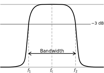
Typically in electronic systems such as filters and communication channels, cutoff frequency applies to an edge in a lowpass, highpass, bandpass, or band-stop characteristic – a frequency characterizing a boundary between a passband and a stopband. It is sometimes taken to be the point in the filter response where a transition band and passband meet, for example, as defined by a 3 dB corner (a frequency for which the output of the circuit is −3 dB of the nominal passband value). Alternatively, a stopband corner frequency may be specified as a point where a transition band and a stopband meet: a frequency for which the attenuation is larger than the required stopband attenuation, which for example may be 30 dB or 100 dB.

In the case of a waveguide or an antenna, the cutoff frequencies correspond to the lower and upper cutoff wavelengths.

Electronics

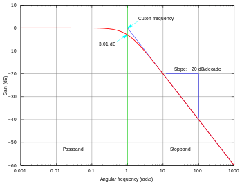
In electronics, cutoff frequency or corner frequency is the frequency either above or below which the power output of a circuit, such as a line, amplifier, or electronic filter has fallen to a given proportion of the power in the passband. Most frequently this proportion is one half the passband power, also referred to as the 3 dB point since a fall of 3 dB corresponds approximately to half power. As a voltage ratio this is a fall to $\scriptstyle {\sqrt {1/2}}\ \approx \ 0.707$ of the passband voltage.^[1] Other ratios besides the 3 dB point may also be relevant, for example see Chebyshev Filters below.

Single-pole transfer function example

The simplest low-pass filter transfer function,

H(s)={\frac {1}{1+\alpha s}},

has a single pole at $s = -1/α$ . The magnitude of this function in the $j ω$ plane is

\left|H(j\omega )\right|=\left|{\frac {1}{1+\alpha j\omega }}\right|={\sqrt {\frac {1}{1+\alpha ^{2}\omega ^{2}}}}.

At cutoff

\left|H(j\omega _{\mathrm {c} })\right|={\frac {1}{\sqrt {2}}}={\sqrt {\frac {1}{1+\alpha ^{2}\omega _{\mathrm {c} }^{2}}}}.

Hence, the cutoff frequency is given by

\omega _{\mathrm {c} }={\frac {1}{\alpha }}.

Where $s$ is the s-plane variable, $ω$ is angular frequency and $j$ is the imaginary unit.

Chebyshev filters

Sometimes other ratios are more convenient than the 3 dB point. For instance, in the case of the Chebyshev filter it is usual to define the cutoff frequency as the point after the last peak in the frequency response at which the level has fallen to the design value of the passband ripple. The amount of ripple in this class of filter can be set by the designer to any desired value, hence the ratio used could be any value.^[2]

Communications

In communications, the term cutoff frequency can mean the frequency below which a radio wave fails to penetrate a layer of the ionosphere at the incidence angle required for transmission between two specified points by reflection from the layer.

Waveguides

The cutoff frequency of an electromagnetic waveguide is the lowest frequency for which a mode will propagate in it. In fiber optics, it is more common to consider the cutoff wavelength, the maximum wavelength that will propagate in an optical fiber or waveguide. The cutoff frequency is found with the characteristic equation of the Helmholtz equation for electromagnetic waves, which is derived from the electromagnetic wave equation by setting the longitudinal wave number equal to zero and solving for the frequency. Thus, any exciting frequency lower than the cutoff frequency will attenuate, rather than propagate. The following derivation assumes lossless walls. The value of c, the speed of light, should be taken to be the group velocity of light in whatever material fills the waveguide.

For a rectangular waveguide, the cutoff frequency is

\omega _{c}=c{\sqrt {\left({\frac {n\pi }{a}}\right)^{2}+\left({\frac {m\pi }{b}}\right)^{2}}},

where the integers $n,m\geq 0$ are the mode numbers, and a and b the lengths of the sides of the rectangle. For TE modes, $n,m\geq 0$ (but $n=m=0$ is not allowed), while for TM modes $n,m\geq 1$ .

The cutoff frequency of the TM₀₁ mode (next higher from dominant mode TE₁₁) in a waveguide of circular cross-section (the transverse-magnetic mode with no angular dependence and lowest radial dependence) is given by

\omega _{c}=c{\frac {\chi _{01}}{r}}=c{\frac {2.4048}{r}},

where $r$ is the radius of the waveguide, and $\chi _{01}$ is the first root of $J_{{0}}(r)$ , the bessel function of the first kind of order 1.

The dominant mode TE₁₁ cutoff frequency is given by

\omega _{c}=c{\frac {\chi _{11}}{r}}=c{\frac {1.8412}{r}}

^[3]

For a single-mode optical fiber, the cutoff wavelength is the wavelength at which the normalized frequency is approximately equal to 2.405.

Mathematical analysis

The starting point is the wave equation (which is derived from the Maxwell equations),

\left(\nabla ^{2}-{\frac {1}{c^{2}}}{\frac {\partial ^{2}}{\partial {t}^{2}}}\right)\psi (\mathbf {r} ,t)=0,

which becomes a Helmholtz equation by considering only functions of the form

\psi (x,y,z,t)=\psi (x,y,z)e^{i\omega t}.

Substituting and evaluating the time derivative gives

(\nabla ^{2}+{\frac {\omega ^{2}}{c^{2}}})\psi (x,y,z)=0.

The function $\psi$ here refers to whichever field (the electric field or the magnetic field) has no vector component in the longitudinal direction - the "transverse" field. It is a property of all the eigenmodes of the electromagnetic waveguide that at least one of the two fields is transverse. The z axis is defined to be along the axis of the waveguide.

The "longitudinal" derivative in the Laplacian can further be reduced by considering only functions of the form

\psi (x,y,z,t)=\psi (x,y)e^{i\left(\omega t-k_{z}z\right)},

where $k_{z}$ is the longitudinal wavenumber, resulting in

(\nabla _{T}^{2}-k_{z}^{2}+{\frac {\omega ^{2}}{c^{2}}})\psi (x,y,z)=0,

where subscript T indicates a 2-dimensional transverse Laplacian. The final step depends on the geometry of the waveguide. The easiest geometry to solve is the rectangular waveguide. In that case the remainder of the Laplacian can be evaluated to its characteristic equation by considering solutions of the form

\psi (x,y,z,t)=\psi _{0}e^{i\left(\omega t-k_{z}z-k_{x}x-k_{y}y\right)}.

Thus for the rectangular guide the Laplacian is evaluated, and we arrive at

{\frac {\omega ^{2}}{c^{2}}}=k_{x}^{2}+k_{y}^{2}+k_{z}^{2}

The transverse wavenumbers can be specified from the standing wave boundary conditions for a rectangular geometry crossection with dimensions a and b:

k_{x}={\frac {n\pi }{a}},

k_{y}={\frac {m\pi }{b}},

where n and m are the two integers representing a specific eigenmode. Performing the final substitution, we obtain

{\frac {\omega ^{2}}{c^{2}}}=\left({\frac {n\pi }{a}}\right)^{2}+\left({\frac {m\pi }{b}}\right)^{2}+k_{z}^{2},

which is the dispersion relation in the rectangular waveguide. The cutoff frequency $\omega _{c}$ is the critical frequency between propagation and attenuation, which corresponds to the frequency at which the longitudinal wavenumber $k_{{z}}$ is zero. It is given by

\omega _{c}=c{\sqrt {\left({\frac {n\pi }{a}}\right)^{2}+\left({\frac {m\pi }{b}}\right)^{2}}}

The wave equations are also valid below the cutoff frequency, where the longitudinal wave number is imaginary. In this case, the field decays exponentially along the waveguide axis and the wave is thus evanescent.

References

↑ Van Valkenburg, M. E. Network Analysis (3rd ed.). pp. 383–384. ISBN 0-13-611095-9. Retrieved 2008-06-22.
↑ Mathaei, Young, Jones Microwave Filters, Impedance-Matching Networks, and Coupling Structures, pp.85-86, McGraw-Hill 1964.
↑ I. C. Hunter, Theory and Design of Microwave Filters, p.214 IET, 2001 ISBN 0-85296-777-2.

This article incorporates public domain material from the General Services Administration document "Federal Standard 1037C" (in support of MIL-STD-188).

External links

This article is issued from Wikipedia - version of the 10/12/2016. The text is available under the Creative Commons Attribution/Share Alike but additional terms may apply for the media files.