Curve resistance (railroad)
In railroad engineering, curve resistance is a part of train resistance, namely the additional rolling resistance a train must overcome when travelling on a curved section of track.[1] Curve resistance is typically measured in per mille, with the correct physical unit being Newton per kilo-Newton or N/kN. Older texts still use the wrong unit of kilogram-force per tonne or kgf/t, which mixes an (outdated) unit of force and a unit of mass. Sometimes also kg/t was used, which confused the resisting force with a mass.
Curve resistance depends on various factors, the most important being the radius and the superelevation of a curve. Since curves are usually banked by superelevation, there will exist some speed at which there will be no sideways force on the train and where therefore curve resistance is minimum. At higher or lower speeds, curve resistance may be a few (or several) times greater.
Approximation formulas
Formulas typically used in railway engineering in general compute the resistance as inversely proportional to the radius of curvature (thus, they neglect the fact that the resistance is dependent on both speed and superelevation). For example, in the USSR, the standard formula is Wr (curve resistance in parts per thousand or kgf/tonne) = 700/R where R is the radius of the curve in meters. Other countries often use the same formula, but with a different numerator-constant. For example, the US used 446/R, Italy 800/R, England 600/R, China 573/R, etc. In Germany, Austria, Switzerland, Czechoslovakia, Hungary, and Romania the term R - b is used in the denominator (instead of just R), where b is some constant. Typically, the expressions used are "Röckl's formula", which uses 650/(R - 55) for R above 300 meters, and 500/(R - 30) for smaller radii. The fact that, at 300 meters, the two values of Röckl's formula differ by more than 30% shows that these formulas are rough estimates at best.
The Russian experiments cited below show that all these formulas are inaccurate. At balancing speed, they give a curve resistance a few times too high (or worse).[2] However, these approximation formulas are still contained in practically all standard railway engineering textbooks. For the US, AREMA American Railway Engineering ..., PDF, p.57 claims that curve resistance is 0.04% per degree of curvature (or 8 lbf/ton or 4 kgf/tonne). Hay's textbook also claims it is independent of superelevation.[3] For Russia in 2011, internet articles use 700/R.[4] [5] [6] German textbooks contain Röckl's formulas.[7]
Speed and cant dependence per Russian experiments
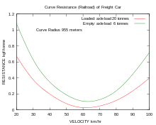
In the 1960s in the Soviet Union curve resistance was found by experiment [8][9] to be highly dependent on both the velocity and the banking of the curve, also known as superelevation or cant, as can bee seen in the graph above. If a train car rounds a curve at balancing speed such that the component of centrifugal force in the lateral direction (towards the outside of the curve and parallel with the plane of the track) is equal to the component of gravitational force in the opposite direction there is very little curve resistance. At such balancing speed there is zero cant deficiency and results in a frictionless banked turn. But deviate from this speed (either higher or lower) and the curve resistance increases due to the unbalance in forces which tends to pull the vehicle sideways (and would be felt by a passenger in a passenger train[10]). Note that for empty rail cars (low wheel loads) the specific curve resistance is higher, similar to the phenomena of higher rolling resistance for empty cars on a straight track.
However, these experiments did not provide usable formulas for curve resistance, because the experiments were, unfortunately, all done on a test track with the same curvature (radius = 955 meters).[11] Therefore, it is not clear how to account for curvature. The Russian experiments plot curve resistance against velocity for various types of railroad cars and various axle loads. The plots all show smooth convex curves with the minimums at balancing speed where the slope of the plotted curve is zero. These plots tend to show curve resistance increasing more rapidly with decreases in velocity below balancing speed, than for increases in velocity (by the same amounts) above balancing speeds. No explanation for this "asymmetrical velocity effect" is to be found in the references cited nor is any explanation found explaining the smooth convex curve plots mentioned above (except for explaining how they were experimentally determined).
That curve resistance is expected to be minimized at balancing speed was also proposed by Schmidt [12] in 1927, but unfortunately the tests he conducted were all at below balancing speed. However his results all show curve resistance decreasing with increasing speed in conformance with this expectation.
Russian method of measuring in 1960s
To experimentally find the curve resistance of a certain railroad freight car with a given load on its axles (partly due to the weight of the freight) the same car was tested both on a curved track and on a straight track. The difference in measured resistance(at the same speed) was assumed to be the curve resistance.[13] To get an average for several cars of the same type, and to reduce the effect of aerodynamic drag, one may test a group of the same type of cars coupled together (a short train without a locomotive). The curved track used in the experiments was the circular test track of the National Scientific Investigation Institute of Railroad Transport (ВНИИЖТ). A single test run can find the train resistance (force) at various velocities by letting the rolling stock being tested coast down from a higher speed to a low speed, while continuously measuring the deceleration and using Newton's second law of motion (force = acceleration*mass) to find the resistance force that is causing the railroad cars to slow.[14] In such calculations, one must take into account the moment of inertia of the car wheels by adding an equivalent mass (of rotating wheels) to the mass of the train consist. Thus the effective mass of a rail car used for Newton's second law, is larger than the car mass as weighed on a car weighing scale. This additional equivalent mass is tantamount to having the mass of each wheel-axle set be located at its radius of gyration See "Inertia Resistance" (for automobile wheels, but it's the same formula for railroad wheels).
Deceleration was measured by measuring the distance traveled (using what might be called a recording odometer or by distance markers placed along the track say every 50 meters), versus time.[15] A division of distance by time results in velocity and then the differences in velocities divided by time gives the deceleration. A sample data sheet shows time (in seconds) being recorded with 3 digits after the decimal point (thousandths of a second).
It turns out that there is no need to know the mass of the rolling stock to find the specific train resistance in kgf/tonne. This unit is force divided by mass which is acceleration per Newton's second law. But one must multiply kilograms of force by g (gravity) to get force in the metric units of Newtons. So the specific force (the result) is the deceleration multiplied by a constant which is 1/g times a factor to account for the equivalent mass due to wheel rotation. Then this specific force in kgf/kg must be multiplied by 1000 to get kgf/tonne since a tonne is 1000 kg.
Formulas which try to account for superelevation (cant)
Астахов proposed the use of a formula which when plotted[16] is in substantial disagreement with the experimental results curves previously mentioned. His formula for curve resistance (in kgf/tonne) is the sum of two terms, the first term being a conventional k/R term (R is the curve radius in meters) with k=200 instead of 700. The second term is directly proportional to (1.5 times) the absolute value of the unbalanced acceleration in the plane of the track and perpendicular to the rail, such lateral acceleration being equal to the centrifugal acceleration , minus the gravitation component opposing this acceleration: g·tan(θ), where θ is the angle of the banking due to superelevation and v is the train velocity in m/s.[17]

See also
External links
References
- ↑ Hay p.142
- ↑ Астахов p.115 Fig. 5.2; p.229, Fig. 5.6
- ↑ Hay, 1982. On p. 142: "experiments have shown no appreciable change in resistance with changes in superelevation" but he cites no reference.
- ↑ See blog where it's erroneously claimed that the "удельного дополнительного сопротивления от радиуса кривой" (specific additional resistance due to the curve radius): wr = 700/Д. (where Д is the radius).
- ↑ See ОПРЕДЕЛЕНИЕ СОПРОТИВЛЕНИЯ В КРИВОЙ ОТ ТРЕНИЯ ГРЕБНЯ КОЛЕСНОЙ ПАРЫ (Finding the resistance in a curve due to flange friction of the wheel pair)by к.т.н. Довбня Н. П., к.т.н. Бондаренко Л. Н., Кислый Д. Н. (к.т.н. stands for "candidate of technical sciences") of Dnepropetrovsk national technical university of railroad transportation (in Russian Wikipedia)
- ↑ Also see Russian Wikipedia uses the old approximation formulas.
- ↑ See e.g. "Bahnbau" by V.Matthews, Teubner, 2007
- ↑ Астахов, pp.115-6, Figs. 5.2, 5.3
- ↑ Деев, p.85, Fig. 5.5
- ↑ Амелин, p.70
- ↑ Астахов, p.115
- ↑ Schmidt, p.32
- ↑ Астахов, pp. 72, 115
- ↑ Астахов, pp. 63-74
- ↑ Астахов pp.63-73
- ↑ Астахов p.119, Fig. 5.6
- ↑ This formula is found in Астахов, bottom of p. 118. Since theta is a small angle, he assumes that cos theta is equal to unity. He approximates "tan theta" by h/S where h is the height of the superelevation of the outside rail and S is the distance between the centers of the pair of rails (something like the rail gauge, but slightly wider). His plot using this formula does show a minimum at the balancing speed (as it should) but the plotted curves of curve resistance suddenly change slope here from negative to positive, in contrast to the experimental curves which are smooth and nearly flat at this point. As velocity increases beyond the balancing speed (cant deficiency), his curves rise much faster than they do for velocities less than the balancing speed, while the experimental curves do just the opposite. Thus one must conclude that his proposed formula is quite erroneous.
- Астахов П.Н. (Russian) "Сопротивление движению железнодорожного подвижного состава" (Resistance to motion of railway rolling stock) Труды ЦНИИ МПС (ISSN 0372-3305). Выпуск 311 (Vol. 311). - Москва: Транспорт, 1966. – 178 pp.
- Амелин, С.В., Андреев, Г.Е.(Russian) "Устройство и эксплуатация пути" (Structure and operation of track). Учебное пособие- Москва: Транспорт, 1986. - 238 pp.
- Деев В.В., Ильин Г.А., Афонин Г.С. (Russian) "Тяга поездов" (Traction of trains). Учебное пособие. - Москва: Транспорт, 1987. - 264 pp.
- Hay, William Walter (1982). Railroad Engineering, 2nd edition. John Wiley and Sons. p. 142. ISBN 0-471-36400-2.
- Newland, D.E "Steering characteristics of bogies" The railway gazette, October 4, 1968, pp. 745–750. Note: "bogie" (UK) = truck (US).
- Schmidt, Edward C.: Freight train curve resistance on a one-degree curve and on a three-degree curve. University of Illinois Bulletin, Vol. XXIV, July 12, 1927 (No. 45).