Block Wiedemann algorithm
The block Wiedemann algorithm for computing kernel vectors of a matrix over a finite field is a generalisation of an algorithm due to Don Coppersmith.
Coppersmith's algorithm
Let  be an
be an  square matrix over some finite field F, let
  be a random vector of length
  , and let
  . Consider the sequence of vectors
 ![S = \left[x, Mx, M^2x, \ldots\right]](../I/m/b5bb71fe6f2cf8b2ea0b1a6249fbd37a.png) obtained by repeatedly multiplying the vector by the matrix ; let
obtained by repeatedly multiplying the vector by the matrix ; let  be any other vector of length , and consider the sequence of finite-field elements
 ![S_y = \left[y \cdot x, y \cdot Mx, y \cdot M^2x \ldots\right]](../I/m/030f80313edfcebb737f9c4c4020f847.png)
We know that the matrix has a minimal polynomial; by the Cayley–Hamilton theorem we know that this polynomial is of degree (which we will call  ) no more than . Say
 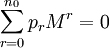 . Then
 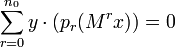 ; so the minimal polynomial of the matrix annihilates the sequence
  and hence
  .
.
But the Berlekamp–Massey algorithm allows us to calculate relatively efficiently some sequence  with
with ![\sum_{i=0}^L q_i S_y[{i+r}]=0 \;\forall \; r](../I/m/f057e8de698dbae7cbc856385f18fbeb.png) . Our hope is that this sequence, which by construction annihilates
. Our hope is that this sequence, which by construction annihilates  , actually annihilates ; so we have
 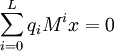 . We then take advantage of the initial definition of
  to say
 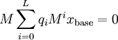 and so
  is a hopefully non-zero kernel vector of .
The block Wiedemann algorithm
The natural implementation of sparse matrix arithmetic on a computer makes it easy to compute the sequence S in parallel for a number of vectors equal to the width of a machine word – indeed, it will normally take no longer to compute for that many vectors than for one. If you have several processors, you can compute the sequence S for a different set of random vectors in parallel on all the computers.
It turns out, by a generalization of the Berlekamp–Massey algorithm to provide a sequence of small matrices, that you can take the sequence produced for a large number of vectors and generate a kernel vector of the original large matrix. You need to compute  for some
  where
where  need to satisfy
 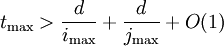 and
and  are a series of vectors of length n; but in practice you can take as a sequence of unit vectors and simply write out the first
  entries in your vectors at each time t.
References
Villard's 1997 research report 'A study of Coppersmith's block Wiedemann algorithm using matrix polynomials' (the cover material is in French but the content in English) is a reasonable description.
Thomé's paper 'Subquadratic computation of vector generating polynomials and improvement of the block Wiedemann algorithm' uses a more sophisticated FFT-based algorithm for computing the vector generating polynomials, and describes a practical implementation with imax = jmax = 4 used to compute a kernel vector of a 484603×484603 matrix of entries modulo 2607−1, and hence to compute discrete logarithms in the field GF(2607).
| ||||||||||||||||||