Blasius boundary layer

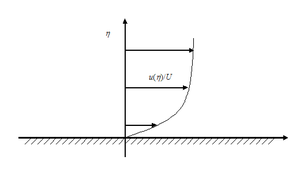
In physics and fluid mechanics, a Blasius boundary layer (named after Paul Richard Heinrich Blasius) describes the steady two-dimensional laminar boundary layer that forms on a semi-infinite plate which is held parallel to a constant unidirectional flow. Falkner and Skan later generalized Blasius' solution to wedge flow, i.e. flows in which the plate is not parallel to the flow.

Prandtl's boundary layer equations

A schematic diagram of the Blasius flow profile. The streamwise velocity component

u(\eta )/U(x)

is shown, as a function of the similarity variable

\eta

Using scaling arguments, Ludwig Prandtl^[1] has argued that about half of the terms in the Navier-Stokes equations are negligible in boundary layer flows (except in a small region near the leading edge of the plate). This leads to a reduced set of equations knows as the boundary layer equations. For steady incompressible flow with constant viscosity and density, these read:

Continuity: ${\dfrac {\partial u}{\partial x}}+{\dfrac {\partial v}{\partial y}}=0$

$x$ -Momentum: $u{\dfrac {\partial u}{\partial x}}+v{\dfrac {\partial u}{\partial y}}=-{\dfrac {1}{\rho }}{\dfrac {\partial p}{\partial x}}+{\nu }{\dfrac {\partial ^{2}u}{\partial y^{2}}}$

$y$ -Momentum: ${\dfrac {\partial p}{\partial y}}=0$

Here the coordinate system is chosen with $x$ pointing parallel to the plate in the direction of the flow and the $y$ coordinate pointing towards the free stream, $u$ and $v$ are the $x$ and $y$ velocity components, $p$ is the pressure, $\rho$ is the density and $\nu$ is the kinematic viscosity.

These three partial differential equations for $u$ , $v$ and $p$ can be reduced to a single equation for $u$ as follows

By integrating the continuity equation over $y$ , $v$ can be expressed as a function of $u$ :

$v=-\int {\dfrac {\partial u}{\partial x}}dy$

The $y$ -momentum equation implies that the pressure in the boundary layer must be equal to that of the free stream for any given $x$ coordinate. Because the velocity profile is flat in the free stream, there are no viscous effects and Bernoulli's law applies:

${\dfrac {p}{\rho }}+{\dfrac {U_{\infty }^{2}}{2}}=$ constant

or, after differentiation:

${\dfrac {1}{\rho }}{\dfrac {dp}{dx}}=-U_{\infty }{\dfrac {dU_{\infty }}{dx}}$

Here $U_\infty$ is the velocity of the free stream. The derivatives are not partials because there is no variation with respect to the $y$ coordinate.

Substitution of these results into the $x$ -momentum equations gives:

u{\dfrac {\partial u}{\partial x}}-{\dfrac {\partial u}{\partial y}}\int {\dfrac {\partial u}{\partial x}}dy=U_{\infty }{\dfrac {dU_{\infty }}{dx}}+{\nu }{\dfrac {\partial ^{2}u}{\partial y^{2}}}

A number of similarity solutions to this equation have been found for various types of flow, including flat plate boundary layers. The term similarity refers to the property that the velocity profiles at different positions in the flow are the same apart from a scaling factor. These solutions are often presented in the form of non-linear ordinary differential equations.

Blasius equation

Blasius^[2] proposed a similarity solution for the case in which the free stream velocity is constant, $\partial U/\partial x=0$ , which corresponds to the boundary layer over a flat plate that is oriented parallel to the free flow. First he introduced the similarity variable

Developing Blasius boundary layer (not to scale). The velocity profile

f'

is shown in red at selected positions along the plate. The blue lines represent, in top to bottom order, the 99% free stream velocity line (

\delta _{99\%},\eta \approx 3.5

), the displacement thickness (

\delta _{*},\eta \approx 1.21

) and

\delta (x)

(

\eta = 1

). See Boundary layer thickness for a more detailed explanation.

\eta ={\dfrac {y}{\delta (x)}}=y{\sqrt {\dfrac {U}{2\nu x}}}

Where $\delta (x)={\sqrt {2\nu x/U}}$ is proportional to the boundary layer thickness. The factor 2 is actually a later addition that, as White^[3] points out, avoids a constant in the final differential equation. Next Blasius proposed the stream function

\psi ={\sqrt {2\nu Ux}}f(\eta )

in which the newly introduced normalized stream function, $f(\eta )$ , is only a function of the similarity variable. This leads directly to the velocity components

u(x,y)={\dfrac {\partial \psi }{\partial y}}=Uf'(\eta )

v(x,y)=-{\dfrac {\partial \psi }{\partial x}}={\sqrt {\dfrac {\nu U}{2x}}}(\eta f'-f)

Where the prime denotes derivation with respect to $\eta$ . Substitution into the momentum equation gives the Blasius equation

f'''+f''f=0

This is a third order non-linear ordinary differential equation which can be solved numerically, e.g. with the shooting method.

The boundary conditions are the no-slip condition

u(x,0)=0\rightarrow f'(0)=0

impermeability of the wall

v(x,0)=0\rightarrow f(0)=0

and the free stream velocity outside the boundary layer

u(x,\infty )=U\rightarrow f'(\infty )=1

Falkner–Skan equation

Wedge flow.

We can generalize the Blasius boundary layer by considering a wedge at an angle of attack $\pi \beta /2$ from some uniform velocity field $U_{0}$ . We then estimate the outer flow to be of the form:

u_{e}(x)=U_{0}\left({\frac {x}{L}}\right)^{m}

Where $L$ is a characteristic length and m is a dimensionless constant. In the Blasius solution, m = 0 corresponding to an angle of attack of zero radians. Thus we can write:

\beta ={\frac {2m}{m+1}}.

As in the Blasius solution, we use a similarity variable $\eta$ to solve the boundary layer equations.

Falkner-Skan boundary layer profiles for selected values of

m

\eta =y{\sqrt {\frac {U_{0}(m+1)}{2\nu L}}}\left({\frac {x}{L}}\right)^{(m-1)/2}

It becomes easier to describe this in terms of its stream function which we write as

\psi =U(x)\delta (x)f(\eta )={\sqrt {\frac {2\nu U_{0}L}{m+1}}}\left({\frac {x}{L}}\right)^{(m+1)/2}f(\eta )

Thus the initial differential equation which was written as follows:

u{\partial u \over \partial x}+v{\partial u \over \partial y}=c^{2}mx^{2m-1}+{\nu }{\partial ^{2}u \over \partial y^{2}}.

Can now be expressed in terms of the non-linear ODE known as the Falkner–Skan equation (named after V. M. Falkner and Sylvia W. Skan^[4]).

f'''+ff''+\beta \left[1-(f')^{2}\right]=0

(note that $m=0$ produces the Blasius equation). See Wilcox 2007.

In 1937 Douglas Hartree revealed that physical solutions exist only in the range $-0.0905\leq m\leq 2$ . Here, m < 0 corresponds to an adverse pressure gradient (often resulting in boundary layer separation) while m > 0 represents a favorable pressure gradient.

External links

- English translation of Prandtl's original paper - NACA Technical Memorandum 452.
- English translation of Blasius' original paper - NACA Technical Memorandum 1256.

References

↑ Prandtl, L. (1904). "Über Flüssigkeitsbewegung bei sehr kleiner Reibung". Verhandlinger 3. Int. Math. Kongr. Heidelberg: 484–491.
↑ Blasius, H. (1908). "Grenzschichten in Flüssigkeiten mit kleiner Reibung". Z. Angew. Math. Phys. 56: 1–37.
↑ White, F.M. (2006). Viscous fluid flow (3 ed.). New York: McGraw-Hill. p. 231. ISBN 007-124493-X.
↑ V. M. Falkner and S. W. Skan, Aero. Res. Coun. Rep. and Mem. no 1314, 1930.

Parlange, J. Y.; Braddock, R. D.; Sander, G. (1981). "Analytical approximations to the solution of the Blasius equation". Acta Mech. 38: 119–125. doi:10.1007/BF01351467.
Pozrikidis, C. (1998). Introduction to Theoretical and Computational Fluid Dynamics. Oxford. ISBN 0-19-509320-8.
Schlichting, H. (2004). Boundary-Layer Theory. Springer. ISBN 3-540-66270-7.
Wilcox, David C. Basic Fluid Mechanics. DCW Industries Inc. 2007
Boyd, John P. (1999), "The Blasius function in the complex plane", Experimental Mathematics, 8 (4): 381–394, doi:10.1080/10586458.1999.10504626, ISSN 1058-6458, MR 1737233

This article is issued from Wikipedia - version of the 9/25/2016. The text is available under the Creative Commons Attribution/Share Alike but additional terms may apply for the media files.