Bivector
In mathematics, a bivector or 2-vector is a quantity in exterior algebra or geometric algebra that extends the idea of scalars and vectors. If a scalar is considered an order zero quantity, and a vector is an order one quantity, then a bivector can be thought of as being of order two. Bivectors have applications in many areas of mathematics and physics. They are related to complex numbers in two dimensions and to both pseudovectors and quaternions in three dimensions. They can be used to generate rotations in any number of dimensions, and are a useful tool for classifying such rotations. They also are used in physics, tying together a number of otherwise unrelated quantities.
Bivectors are generated by the exterior product on vectors: given two vectors a and b, their exterior product a ∧ b is a bivector, as is the sum of any bivectors. Not all bivectors can be generated as a single exterior product. More precisely, a bivector that can be expressed as an exterior product is called simple; in up to three dimensions all bivectors are simple, but in higher dimensions this is not the case.[1] The exterior product of two vectors is antisymmetric, so b ∧ a is the negation of the bivector a ∧ b, producing the opposite orientation, and a ∧ a is the zero bivector.
Geometrically, a simple bivector can be interpreted as an oriented plane segment, much as vectors can be thought of as directed line segments.[3] The bivector a ∧ b has a magnitude equal to the area of the parallelogram with edges a and b, has the attitude of the plane spanned by a and b, and has orientation being the sense of the rotation that would align a with b.[3][4]
History
The bivector was first defined in 1844 by German mathematician Hermann Grassmann in exterior algebra as the result of the exterior product of two vectors. Around the same time in 1843 in Ireland William Rowan Hamilton discovered quaternions. It was not until English mathematician William Kingdon Clifford in 1888 added the geometric product to Grassmann's algebra, incorporating the ideas of both Hamilton and Grassmann, and founded Clifford algebra, that the bivector as it is known today was fully understood.
Around this time Josiah Willard Gibbs and Oliver Heaviside developed vector calculus, which included separate cross product and dot products that were derived from quaternion multiplication.[5][6][7] The success of vector calculus, and of the book Vector Analysis by Gibbs and Wilson, had the effect that the insights of Hamilton and Clifford were overlooked for a long time, since much of 20th century mathematics and physics was formulated in vector terms. Gibbs used vectors to fill the role of bivectors in three dimensions, and used "bivector" to describe an unrelated quantity, a use that has sometimes been copied.[8][9][10]
Today the bivector is largely studied as a topic in geometric algebra, a Clifford algebra over real or complex vector spaces with a nondegenerate quadratic form. Its resurgence was led by David Hestenes who, along with others, applied geometric algebra to a range of new applications in physics.[11]
Derivation
For this article the bivector will be considered only in real geometric algebras. This in practice is not much of a restriction, as all useful applications are drawn from such algebras. Also unless otherwise stated, all examples have a Euclidean metric and so a positive-definite quadratic form.
Geometric algebra and the geometric product
The bivector arises from the definition of the geometric product over a vector space. For vectors a, b and c, the geometric product on vectors is defined as follows:

Left and right distributivity:


Contraction:

Where Q is the quadratic form, |a| is the magnitude of a and ϵa is the signature of the vector. For a space with Euclidean metric ϵa is 1 so can be omitted, and the contraction condition becomes:

The interior product
From associativity a(ab) = a2b, a scalar times b. When b is not parallel to and hence not a scalar multiple of a, ab cannot be a scalar. But

is a sum of scalars and so a scalar. From the law of cosines on the triangle formed by the vectors its value is |a||b|cosθ, where θ is the angle between the vectors. It is therefore identical to the interior product between two vectors, and is written the same way,

It is symmetric, scalar valued, and can be used to determine the angle between two vectors: in particular if a and b are orthogonal the product is zero.
The exterior product
Just as the interior product can be formulated as the symmetric part of the geometric product another quantity, the exterior product can be formulated as its antisymmetric part:

It is antisymmetric in a and b

and by addition:

That is, the geometric product is the sum of the symmetric interior product and antisymmetric exterior product.
To examine the nature of a ∧ b, consider the formula

which using the Pythagorean trigonometric identity gives the value of (a ∧ b)2

With a negative square it cannot be a scalar or vector quantity, so it is a new sort of object, a bivector. It has magnitude | a | | b | | sinθ |, where θ is the angle between the vectors, and so is zero for parallel vectors.
To distinguish them from vectors, bivectors are written here with bold capitals, for example:

although other conventions are used, in particular as vectors and bivectors are both elements of the geometric algebra.
Properties
The space Λ2ℝn
The algebra generated by the geometric product is the geometric algebra over the vector space. For a Euclidean vector space it is written or Cℓn(ℝ), where n is the dimension of the vector space ℝn. Cℓn is both a vector space and an algebra, generated by all the products between vectors in ℝn, so it contains all vectors and bivectors. More precisely as a vector space it contains the vectors and bivectors as linear subspaces, though not subalgebras. The space of all bivectors is written Λ2ℝn.[12]

The even subalgebra
The subalgebra generated by the bivectors is the even subalgebra of the geometric algebra, written Cℓ +
n . This algebra results from considering all products of scalars and bivectors generated by the geometric product. It has dimension 2n − 1, and contains Λ2ℝn as a linear subspace with dimension 1/2n(n − 1) (a triangular number). In two and three dimensions the even subalgebra contains only scalars and bivectors, and each is of particular interest. In two dimensions the even subalgebra is isomorphic to the complex numbers, ℂ, while in three it is isomorphic to the quaternions, ℍ. More generally the even subalgebra can be used to generate rotations in any dimension, and can be generated by bivectors in the algebra.
Magnitude
As noted in the previous section the magnitude of a simple bivector, that is one that is the exterior product of two vectors a and b, is |a||b|sin θ, where θ is the angle between the vectors. It is written |B|, where B is the bivector.
For general bivectors the magnitude can be calculated by taking the norm of the bivector considered as a vector in the space Λ2ℝn. If the magnitude is zero then all the bivector's components are zero, and the bivector is the zero bivector which as an element of the geometric algebra equals the scalar zero.
Unit bivectors
A unit bivector is one with unit magnitude. It can be derived from any non-zero bivector by dividing the bivector by its magnitude, that is

Of particular interest are the unit bivectors formed from the products of the standard basis. If ei and ej are distinct basis vectors then the product ei ∧ ej is a bivector. As the vectors are orthogonal this is just eiej, written eij, with unit magnitude as the vectors are unit vectors. The set of all such bivectors form a basis for Λ2ℝn. For instance in four dimensions the basis for Λ2ℝ4 is (e1e2, e1e3, e1e4, e2e3, e2e4, e3e4) or (e12, e13, e14, e23, e24, e34).[13]
Simple bivectors
The exterior product of two vectors is a bivector, but not all bivectors are exterior products of two vectors. For example, in four dimensions the bivector

cannot be written as the exterior product of two vectors. A bivector that can be written as the exterior product of two vectors is simple. In two and three dimensions all bivectors are simple, but not in four or more dimensions; in four dimensions every bivector is the sum of at most two exterior products. A bivector has a real square if and only if it is simple, and only simple bivectors can be represented geometrically by an oriented plane area.[1]
Product of two bivectors
The geometric product of two bivectors, A and B, is

The quantity A · B is the scalar valued interior product, while A ∧ B is the grade 4 exterior product that arises in four or more dimensions. The quantity A × B is the bivector valued commutator product, given by

The space of bivectors Λ2ℝn are a Lie algebra over ℝ, with the commutator product as the Lie bracket. The full geometric product of bivectors generates the even subalgebra.
Of particular interest is the product of a bivector with itself. As the commutator product is antisymmetric the product simplifies to

If the bivector is simple the last term is zero and the product is the scalar valued A · A, which can be used as a check for simplicity. In particular the exterior product of bivectors only exists in four or more dimensions, so all bivectors in two and three dimensions are simple.[1]
Two dimensions
When working with coordinates in geometric algebra it is usual to write the basis vectors as (e1, e2, ...), a convention that will be used here.
A vector in real two-dimensional space ℝ2 can be written a = a1e1 + a2e2, where a1 and a2 are real numbers, e1 and e2 are orthonormal basis vectors. The geometric product of two such vectors is

This can be split into the symmetric, scalar valued, interior product and an antisymmetric, bivector valued exterior product:

All bivectors in two dimensions are of this form, that is multiples of the bivector e1e2, written e12 to emphasise it is a bivector rather than a vector. The magnitude of e12 is 1, with

so it is called the unit bivector. The term unit bivector can be used in other dimensions but it is only uniquely defined (up to a sign) in two dimensions and all bivectors are multiples of e12. As the highest grade element of the algebra e12 is also the pseudoscalar which is given the symbol i.
Complex numbers
With the properties of negative square and unit magnitude, the unit bivector can be identified with the imaginary unit from complex numbers. The bivectors and scalars together form the even subalgebra of the geometric algebra, which is isomorphic to the complex numbers ℂ. The even subalgebra has basis (1, e12), the whole algebra has basis (1, e1, e2, e12).
The complex numbers are usually identified with the coordinate axes and two-dimensional vectors, which would mean associating them with the vector elements of the geometric algebra. There is no contradiction in this, as to get from a general vector to a complex number an axis needs to be identified as the real axis, e1 say. This multiplies by all vectors to generate the elements of even subalgebra.
All the properties of complex numbers can be derived from bivectors, but two are of particular interest. First as with complex numbers products of bivectors and so the even subalgebra are commutative. This is only true in two dimensions, so properties of the bivector in two dimensions that depend on commutativity do not usually generalise to higher dimensions.
Second a general bivector can be written

where θ is a real number. Putting this into the Taylor series for the exponential map and using the property e122 = −1 results in a bivector version of Euler's formula,

which when multiplied by any vector rotates it through an angle θ about the origin:

The product of a vector with a bivector in two dimensions is anticommutative, so the following products all generate the same rotation

Of these the last product is the one that generalises into higher dimensions. The quantity needed is called a rotor and is given the symbol R, so in two dimensions a rotor that rotates through angle θ can be written

and the rotation it generates is[15]

Three dimensions
In three dimensions the geometric product of two vectors is

This can be split into the symmetric, scalar valued, interior product and the antisymmetric, bivector valued, exterior product:

In three dimensions all bivectors are simple and so the result of an exterior product. The unit bivectors e23, e31 and e12 form a basis for the space of bivectors Λ2ℝ3, which itself a three-dimensional linear space. So if a general bivector is:

they can be added like vectors

while when multiplied they produce the following

which can be split into symmetric scalar and antisymmetric bivector parts as follows

The exterior product of two bivectors in three dimensions is zero.
A bivector B can be written as the product of its magnitude and a unit bivector, so writing β for |B| and using the Taylor series for the exponential map it can be shown that

This is another version of Euler's formula, but with a general bivector in three dimensions. Unlike in two dimensions bivectors are not commutative so properties that depend on commutativity do not apply in three dimensions. For example, in general eA + B ≠ eAeB in three (or more) dimensions.
The full geometric algebra in three dimensions, Cℓ3(ℝ), has basis (1, e1, e2, e3, e23, e31, e12, e123). The element e123 is a trivector and the pseudoscalar for the geometry. Bivectors in three dimensions are sometimes identified with pseudovectors[16] to which they are related, as discussed below.
Quaternions
Bivectors are not closed under the geometric product, but the even subalgebra is. In three dimensions it consists of all scalar and bivector elements of the geometric algebra, so a general element can be written for example a + A, where a is the scalar part and A is the bivector part. It is written Cℓ +
3 and has basis (1, e23, e31, e12). The product of two general elements of the even subalgebra is

The even subalgebra, that is the algebra consisting of scalars and bivectors, is isomorphic to the quaternions, ℍ. This can be seen by comparing the basis to the quaternion basis, or from the above product which is identical to the quaternion product, except for a change of sign which relates to the negative products in the bivector interior product A · B. Other quaternion properties can be similarly related to or derived from geometric algebra.
This suggests that the usual split of a quaternion into scalar and vector parts would be better represented as a split into scalar and bivector parts; if this is done the quaternion product is merely the geometric product. It also relates quaternions in three dimensions to complex numbers in two, as each is isomorphic to the even subalgebra for the dimension, a relationship that generalises to higher dimensions.
Rotation vector
The rotation vector, from the axis-angle representation of rotations, is a compact way of representing rotations in three dimensions. In its most compact form, it consists of a vector, the product of a unit vector ω that is the axis of rotation with the (signed) angle of rotation θ, so that the magnitude of the overall rotation vector θω equals the (unsigned) rotation angle.
The quaternion associated with the rotation is

In geometric algebra the rotation is represented by a bivector. This can be seen in its relation to quaternions. Let Ω be a unit bivector in the plane of rotation, and let θ be the angle of rotation. Then the rotation bivector is Ωθ. The quaternion closely corresponds to the exponential of half of the bivector Ωθ. That is, the components of the quaternion correspond to the scalar and bivector parts of the following expression:

The exponential can be defined in terms of its power series, and easily evaluated using the fact that Ω squared is -1.
So rotations can be represented by bivectors. Just as quaternions are elements of the geometric algebra, they are related by the exponential map in that algebra.
Rotors
The bivector Ωθ generates a rotation through the exponential map. The even elements generated rotate a general vector in three dimensions in the same way as quaternions:

As to two dimensions the quantity eΩθ is called a rotor and written R. The quantity e−Ωθ is then R−1, and they generate rotations as follows
This is identical to two dimensions, except here rotors are four-dimensional objects isomorphic to the quaternions. This can be generalised to all dimensions, with rotors, elements of the even subalgebra with unit magnitude, being generated by the exponential map from bivectors. They form a double cover over the rotation group, so the rotors R and −R represent the same rotation.
Matrices
Bivectors are isomorphic to skew-symmetric matrices; the general bivector B23e23 + B31e31 + B12e12 maps to the matrix

This multiplied by vectors on both sides gives the same vector as the product of a vector and bivector minus the outerproduct; an example is the angular velocity tensor.
Skew symmetric matrices generate orthogonal matrices with determinant 1 through the exponential map. In particular the exponent of a bivector associated with a rotation is a rotation matrix, that is the rotation matrix MR given by the above skew-symmetric matrix is

The rotation described by MR is the same as that described by the rotor R given by

and the matrix MR can be also calculated directly from rotor R:

Bivectors are related to the eigenvalues of a rotation matrix. Given a rotation matrix M the eigenvalues can calculated by solving the characteristic equation for that matrix 0 = det(M − λI). By the fundamental theorem of algebra this has three roots, but only one real root as there is only one eigenvector, the axis of rotation. The other roots must be a complex conjugate pair. They have unit magnitude so purely imaginary logarithms, equal to the magnitude of the bivector associated with the rotation, which is also the angle of rotation. The eigenvectors associated with the complex eigenvalues are in the plane of the bivector, so the exterior product of two non-parallel eigenvectors result in the bivector, or at least a multiple of it.
Axial vectors
The rotation vector is an example of an axial vector. Axial vectors, or pseudovectors, are vectors with the special feature that their coordinates undergo a sign change relative to the usual vectors (also called "polar vectors") under inversion through the origin, reflection in a plane, or other orientation-reversing linear transformation.[17] Examples include quantities like torque, angular momentum and vector magnetic fields. Quantities that would use axial vectors in vector algebra are properly represented by bivectors in geometric algebra.[18] More precisely, if an underlying orientation is chosen, the axial vectors are naturally identified with the usual vectors; the Hodge dual then gives the isomorphism between axial vectors and bivectors, so each axial vector is associated with a bivector and vice versa; that is

where ∗ indicates the Hodge dual. Note that if the underlying orientation is reversed by inversion through the origin, both the identification of the axial vectors with the usual vectors and the Hodge dual change sign, but the bivectors don't budge. Alternately, using the unit pseudoscalar in Cℓ3(ℝ), i = e1e2e3 gives

This is easier to use as the product is just the geometric product. But it is antisymmetric because (as in two dimensions) the unit pseudoscalar i squares to −1, so a negative is needed in one of the products.
This relationship extends to operations like the vector valued cross product and bivector valued exterior product, as when written as determinants they are calculated in the same way:

so are related by the Hodge dual:

Bivectors have a number of advantages over axial vectors. They better disambiguate axial and polar vectors, that is the quantities represented by them, so it is clearer which operations are allowed and what their results are. For example, the inner product of a polar vector and an axial vector resulting from the cross product in the triple product should result in a pseudoscalar, a result which is more obvious if the calculation is framed as the exterior product of a vector and bivector. They generalises to other dimensions; in particular bivectors can be used to describe quantities like torque and angular momentum in two as well as three dimensions. Also, they closely match geometric intuition in a number of ways, as seen in the next section.[19]
Geometric interpretation
As suggested by their name and that of the algebra, one of the attractions of bivectors is that they have a natural geometric interpretation. This can be described in any dimension but is best done in three where parallels can be drawn with more familiar objects, before being applied to higher dimensions. In two dimensions the geometric interpretation is trivial, as the space is two-dimensional so has only one plane, and all bivectors are associated with it differing only by a scale factor.
All bivectors can be interpreted as planes, or more precisely as directed plane segments. In three dimensions there are three properties of a bivector that can be interpreted geometrically:
- The arrangement of the plane in space, precisely the attitude of the plane (or alternately the rotation, geometric orientation or gradient of the plane), is associated with the ratio of the bivector components. In particular the three basis bivectors, e23, e31 and e12, or scalar multiples of them, are associated with the yz-plane, xz-plane and xy-plane respectively.
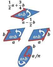
- The magnitude of the bivector is associated with the area of the plane segment. The area does not have a particular shape so any shape can be used. It can even be represented in other ways, such as by an angular measure. But if the vectors are interpreted as lengths the bivector is usually interpreted as an area with the same units, as follows.
- Like the direction of a vector a plane associated with a bivector has a direction, a circulation or a sense of rotation in the plane, which takes two values seen as clockwise and counterclockwise when viewed from viewpoint not in the plane. This is associated with a change of sign in the bivector, that is if the direction is reversed the bivector is negated. Alternately if two bivectors have the same attitude and magnitude but opposite directions then one is the negative of the other.
- If imagined as a 2d parallelogram, with vector's origin at 0, then signed area is the determinant of the vectors' Cartesian coordinates ().[20]

In three dimensions all bivectors can be generated by the exterior product of two vectors. If the bivector B = a ∧ b then the magnitude of B is

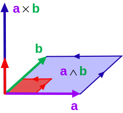
where θ is the angle between the vectors. This is the area of the parallelogram with edges a and b, as shown in the diagram. One interpretation is that the area is swept out by b as it moves along a. The exterior product is antisymmetric, so reversing the order of a and b to make a move along b results in a bivector with the opposite direction that is the negative of the first. The plane of bivector a ∧ b contains both a and b so they are both parallel to the plane.
Bivectors and axial vectors are related by Hodge dual. In a real vector space the Hodge dual relates a subspace to its orthogonal complement, so if a bivector is represented by a plane then the axial vector associated with it is simply the plane's surface normal. The plane has two normals, one on each side, giving the two possible orientations for the plane and bivector.

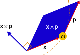
This relates the cross product to the exterior product. It can also be used to represent physical quantities, like torque and angular momentum. In vector algebra they are usually represented by vectors, perpendicular to the plane of the force, linear momentum or displacement that they are calculated from. But if a bivector is used instead the plane is the plane of the bivector, so is a more natural way to represent the quantities and the way they act. It also unlike the vector representation generalises into other dimensions.
The product of two bivectors has a geometric interpretation. For non-zero bivectors A and B the product can be split into symmetric and antisymmetric parts as follows:

Like vectors these have magnitudes | A · B | = | A || B | cos θ and | A × B | = | A || B | sin θ, where θ is the angle between the planes. In three dimensions it is the same as the angle between the normal vectors dual to the planes, and it generalises to some extent in higher dimensions.
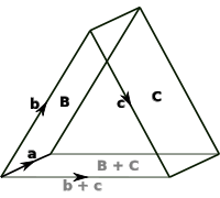
Bivectors can be added together as areas. Given two non-zero bivectors B and C in three dimensions it is always possible to find a vector that is contained in both, a say, so the bivectors can be written as exterior products involving a:

This can be interpreted geometrically as seen in the diagram: the two areas sum to give a third, with the three areas forming faces of a prism with a, b, c and b + c as edges. This corresponds to the two ways of calculating the area using the distributivity of the exterior product:

This only works in three dimensions as it is the only dimension where a vector parallel to both bivectors must exist. In higher dimensions bivectors generally are not associated with a single plane, or if they are (simple bivectors) two bivectors may have no vector in common, and so sum to a non-simple bivector.
Four dimensions
In four dimensions the basis elements for the space Λ2ℝ4 of bivectors are (e12, e13, e14, e23, e24, e34), so a general bivector is of the form

Orthogonality
In four dimensions the Hodge dual of a bivector is a bivector, and the space Λ2ℝ4 is dual to itself. Normal vectors are not unique, instead every plane is orthogonal to all the vectors in its Hodge dual space. This can be used to partition the bivectors into two 'halves', in the following way. We have three pairs of orthogonal bivectors: (e12, e34), (e13, e24) and (e14, e23). There are four distinct ways of picking one bivector from each of the first two pairs, and once these first two are picked their sum yields the third bivector from the other pair. For example, (e12, e13, e14) and (e23, e24, e34).
Simple bivectors in 4D
In four dimensions bivectors are generated by the exterior product of vectors in ℝ4, but with one important difference from ℝ3 and ℝ2. In four dimensions not all bivectors are simple. There are bivectors such as e12 + e34 that cannot be generated by the external product of two vectors. This also means they do not have a real, that is scalar, square. In this case

The element e1234 is the pseudoscalar in Cℓ4, distinct from the scalar, so the square is non-scalar.
All bivectors in four dimensions can be generated using at most two exterior products and four vectors. The above bivector can be written as

Similarly, every bivector can be written as the sum of two simple bivectors. It is useful to choose two orthogonal bivectors for this, and this is always possible to do. Moreover, for a generic bivector the choice of simple bivectors is unique, that is, there is only one way to decompose into orthogonal bivectors; the only exception is when the two orthogonal bivectors have equal magnitudes (as in the above example): in this case the decomposition is not unique.[1] The decomposition is always unique in the case of simple bivectors, with the added bonus that one of the orthogonal parts is zero.
Rotations in ℝ4
As in three dimensions bivectors in four dimension generate rotations through the exponential map, and all rotations can be generated this way. As in three dimensions if B is a bivector then the rotor R is eB/2 and rotations are generated in the same way:

The rotations generated are more complex though. They can be categorised as follows:
- simple rotations are those that fix a plane in 4D, and rotate by an angle "about" this plane.
- double rotations have only one fixed point, the origin, and rotate through two angles about two orthogonal planes. In general the angles are different and the planes are uniquely specified
- isoclinic rotations are double rotations where the angles of rotation are equal. In this case the planes about which the rotation is taking place are not unique.
These are generated by bivectors in a straightforward way. Simple rotations are generated by simple bivectors, with the fixed plane the dual or orthogonal to the plane of the bivector. The rotation can be said to take place about that plane, in the plane of the bivector. All other bivectors generate double rotations, with the two angles of the rotation equalling the magnitudes of the two simple bivectors the non-simple bivector is composed of. Isoclinic rotations arise when these magnitudes are equal, in which case the decomposition into two simple bivectors is not unique.[21]
Bivectors in general do not commute, but one exception is orthogonal bivectors and exponents of them. So if the bivector B = B1 + B2, where B1 and B2 are orthogonal simple bivectors, is used to generate a rotation it decomposes into two simple rotations that commute as follows:

It is always possible to do this as all bivectors can be expressed as sums of orthogonal bivectors.
Spacetime rotations
Spacetime is a mathematical model for our universe used in special relativity. It consists of three space dimensions and one time dimension combined into a single four-dimensional space. It is naturally described using geometric algebra and bivectors, with the Euclidean metric replaced by a Minkowski metric. That algebra is identical to that of Euclidean space, except the signature is changed, so

(Note the order and indices above are not universal – here e4 is the time-like dimension). The geometric algebra is Cℓ3,1(ℝ), and the subspace of bivectors is Λ2ℝ3,1.
The simple bivectors are of two types. The simple bivectors e23, e31 and e12 have negative squares and span the bivectors of the three-dimensional subspace corresponding to Euclidean space, ℝ3. These bivectors generate ordinary rotations in ℝ3.
The simple bivectors e14, e24 and e34 have positive squares and as planes span a space dimension and the time dimension. These also generate rotations through the exponential map, but instead of trigonometric functions, hyperbolic functions are needed, which generates a rotor as follows:

where Ω is the bivector (e14, etc.), identified via the metric with an antisymmetric linear transformation of ℝ3,1. These are Lorentz boosts, expressed in a particularly compact way, using the same kind of algebra as in ℝ3 and ℝ4.
In general all spacetime rotations are generated from bivectors through the exponential map, that is, a general rotor generated by bivector A is of the form

The set of all rotations in spacetime form the Lorentz group, and from them most of the consequences of special relativity can be deduced. More generally this show how transformations in Euclidean space and spacetime can all be described using the same kind of algebra.
Maxwell's equations
(Note: in this section traditional 3-vectors are indicated by lines over the symbols and spacetime vector and bivectors by bold symbols, with the vectors J and A exceptionally in uppercase)
Maxwell's equations are used in physics to describe the relationship between electric and magnetic fields. Normally given as four differential equations they have a particularly compact form when the fields are expressed as a spacetime bivector from Λ2ℝ3,1. If the electric and magnetic fields in ℝ3 are E and B then the electromagnetic bivector is

where e4 is again the basis vector for the time-like dimension and c is the speed of light. The product Be123 yields the bivector that is Hodge dual to B in three dimensions, as discussed above, while Ee4 as a product of orthogonal vectors is also bivector valued. As a whole it is the electromagnetic tensor expressed more compactly as a bivector, and is used as follows. First it is related to the 4-current J, a vector quantity given by

where j is current density and ρ is charge density. They are related by a differential operator ∂, which is

The operator ∇ is a differential operator in geometric algebra, acting on the space dimensions and given by ∇M = ∇·M + ∇∧M. When applied to vectors ∇·M is the divergence and ∇∧M is the curl but with a bivector rather than vector result, that is dual in three dimensions to the curl. For general quantity M they act as grade lowering and raising differential operators. In particular if M is a scalar then this operator is just the gradient, and it can be thought of as a geometric algebraic del operator.
Together these can be used to give a particularly compact form for Maxwell's equations in a vacuum:

This when decomposed according to geometric algebra, using geometric products which have both grade raising and grade lowering effects, is equivalent to Maxwell's four equations. This is the form in a vacuum, but the general form is only a little more complex. It is also related to the electromagnetic four-potential, a vector A given by

where A is the vector magnetic potential and V is the electric potential. It is related to the electromagnetic bivector as follows

using the same differential operator ∂.[22]
Higher dimensions
As has been suggested in earlier sections much of geometric algebra generalises well into higher dimensions. The geometric algebra for the real space ℝn is Cℓn(ℝ), and the subspace of bivectors is Λ2ℝn.
The number of simple bivectors needed to form a general bivector rises with the dimension, so for n odd it is (n − 1) / 2, for n even it is n / 2. So for four and five dimensions only two simple bivectors are needed but three are required for six and seven dimensions. For example, in six dimensions with standard basis (e1, e2, e3, e4, e5, e6) the bivector

is the sum of three simple bivectors but no less. As in four dimensions it is always possible to find orthogonal simple bivectors for this sum.
Rotations in higher dimensions
As in three and four dimensions rotors are generated by the exponential map, so

is the rotor generated by bivector B. Simple rotations, that take place in a plane of rotation around a fixed blade of dimension (n − 2) are generated by simple bivectors, while other bivectors generate more complex rotations which can be described in terms of the simple bivectors they are sums of, each related to a plane of rotation. All bivectors can be expressed as the sum of orthogonal and commutative simple bivectors, so rotations can always be decomposed into a set of commutative rotations about the planes associated with these bivectors. The group of the rotors in n dimensions is the spin group, Spin(n).
One notable feature, related to the number of simple bivectors and so rotation planes, is that in odd dimensions every rotation has a fixed axis – it is misleading to call it an axis of rotation as in higher dimensions rotations are taking place in multiple planes orthogonal to it. This is related to bivectors, as bivectors in odd dimensions decompose into the same number of bivectors as the even dimension below, so have the same number of planes, but one extra dimension. As each plane generates rotations in two dimensions in odd dimensions there must be one dimension, that is an axis, that is not being rotated.[23]
Bivectors are also related to the rotation matrix in n dimensions. As in three dimensions the characteristic equation of the matrix can be solved to find the eigenvalues. In odd dimensions this has one real root, with eigenvector the fixed axis, and in even dimensions it has no real roots, so either all or all but one of the roots are complex conjugate pairs. Each pair is associated with a simple component of the bivector associated with the rotation. In particular the log of each pair is ± the magnitude, while eigenvectors generated from the roots are parallel to and so can be used to generate the bivector. In general the eigenvalues and bivectors are unique, and the set of eigenvalues gives the full decomposition into simple bivectors; if roots are repeated then the decomposition of the bivector into simple bivectors is not unique.
Projective geometry
Geometric algebra can be applied to projective geometry in a straightforward way. The geometric algebra used is Cℓn(ℝ), n ≥ 3, the algebra of the real vector space ℝn. This is used to describe objects in the real projective space ℝℙn − 1. The non-zero vectors in Cℓn(ℝ) or ℝn are associated with points in the projective space so vectors that differ only by a scale factor, so their exterior product is zero, map to the same point. Non-zero simple bivectors in Λ2ℝn represent lines in ℝℙn − 1, with bivectors differing only by a (positive or negative) scale factor representing the same line.
A description of the projective geometry can be constructed in the geometric algebra using basic operations. For example, given two distinct points in ℝℙn − 1 represented by vectors a and b the line between them is given by a ∧ b (or b ∧ a). Two lines intersect in a point if A ∧ B = 0 for their bivectors A and B. This point is given by the vector

The operation "⋁" is the meet, which can be defined as above in terms of the join, J = A ∧ B for non-zero A ∧ B. Using these operations projective geometry can be formulated in terms of geometric algebra. For example, given a third (non-zero) bivector C the point p lies on the line given by C if and only if

So the condition for the lines given by A, B and C to be collinear is

which in Cℓ3(ℝ) and ℝℙ2 simplifies to

where the angle brackets denote the scalar part of the geometric product. In the same way all projective space operations can be written in terms of geometric algebra, with bivectors representing general lines in projective space, so the whole geometry can be developed using geometric algebra.[14]
Tensors and matrices
As noted above a bivector can be written as a skew-symmetric matrix, which through the exponential map generates a rotation matrix that describes the same rotation as the rotor, also generated by the exponential map but applied to the vector. But it is also used with other bivectors such as the angular velocity tensor and the electromagnetic tensor, respectively a 3×3 and 4×4 skew-symmetric matrix or tensor.
Real bivectors in Λ2ℝn are isomorphic to n×n skew-symmetric matrices, or alternately to antisymmetric tensors of order 2 on ℝn. While bivectors are isomorphic to vectors (via the dual) in three dimensions they can be represented by skew-symmetric matrices in any dimension. This is useful for relating bivectors to problems described by matrices, so they can be re-cast in terms of bivectors, given a geometric interpretation, then often solved more easily or related geometrically to other bivector problems.[24]
More generally every real geometric algebra is isomorphic to a matrix algebra. These contain bivectors as a subspace, though often in a way which is not especially useful. These matrices are mainly of interest as a way of classifying Clifford algebras.[25]
See also
| Look up bivector in Wiktionary, the free dictionary. |
Notes
- 1 2 3 4 Lounesto (2001) p. 87
- 1 2 Leo Dorst; Daniel Fontijne; Stephen Mann (2009). Geometric Algebra for Computer Science: An Object-Oriented Approach to Geometry (2nd ed.). Morgan Kaufmann. p. 32. ISBN 0-12-374942-5.
The algebraic bivector is not specific on shape; geometrically it is an amount of oriented area in a specific plane, that's all.
- 1 2 David Hestenes (1999). New foundations for classical mechanics: Fundamental Theories of Physics (2nd ed.). Springer. p. 21. ISBN 0-7923-5302-1.
- ↑ Lounesto (2001) p. 33
- ↑ Karen Hunger Parshall; David E. Rowe (1997). The Emergence of the American Mathematical Research Community, 1876–1900. American Mathematical Society. p. 31 ff. ISBN 0-8218-0907-5.
- ↑ Rida T. Farouki (2007). "Chapter 5: Quaternions". Pythagorean-hodograph curves: algebra and geometry inseparable. Springer. p. 60 ff. ISBN 3-540-73397-3.
- ↑ A discussion of quaternions from these years is Alexander McAulay (1911). "Quaternions". The encyclopædia britannica: a dictionary of arts, sciences, literature and general information. Vol. 22 (11th ed.). Cambridge University Press. p. 718 et seq.
- ↑ Josiah Willard Gibbs; Edwin Bidwell Wilson (1901). Vector analysis: a text-book for the use of students of mathematics and physics. Yale University Press. p. 481 ff.
- ↑ Philippe Boulanger; Michael A. Hayes (1993). Bivectors and waves in mechanics and optics. Springer. ISBN 0-412-46460-8.
- ↑ PH Boulanger & M Hayes (1991). "Bivectors and inhomogeneous plane waves in anisotropic elastic bodies". In Julian J. Wu; Thomas Chi-tsai Ting & David M. Barnett. Modern theory of anisotropic elasticity and applications. Society for Industrial and Applied Mathematics (SIAM). p. 280 et seq. ISBN 0-89871-289-0.
- ↑ David Hestenes. op. cit. p. 61. ISBN 0-7923-5302-1.
- 1 2 Lounesto (2001) p. 35
- ↑ Lounesto (2001) p. 86
- 1 2 Hestenes, David; Ziegler, Renatus (1991). "Projective Geometry with Clifford Algebra" (PDF). Acta Applicandae Mathematicae. 23: 25–63. doi:10.1007/bf00046919.
- ↑ Lounesto (2001) p.29
- ↑ William E Baylis (1994). Theoretical methods in the physical sciences: an introduction to problem solving using Maple V. Birkhäuser. p. 234, see footnote. ISBN 0-8176-3715-X.
The terms axial vector and pseudovector are often treated as synonymous, but it is quite useful to be able to distinguish a bivector (...the pseudovector) from its dual (...the axial vector).
- ↑ In strict mathematical terms, axial vectors are an n-dimensional vector space equipped with the usual structure group GL(n,R), but with the nonstandard representation A → A det(A)/|det(A)|.
- ↑ Chris Doran; Anthony Lasenby (2003). Geometric algebra for physicists. Cambridge University Press. p. 56. ISBN 0-521-48022-1.
- ↑ Lounesto (2001) pp. 37–39
- ↑ WildLinAlg episode 4, Norman J Wildberger, Univ. of New South Wales, 2010, lecture via youtube
- ↑ Lounesto (2001) pp. 89–90
- ↑ Lounesto (2001) pp. 109–110
- ↑ Lounesto (2001) p.222
- ↑ Lounesto (2001) p. 193
- ↑ Lounesto (2001) p. 217
General references
- Leo Dorst; Daniel Fontijne; Stephen Mann (2009). "§ 2.3.3 Visualizing bivectors". Geometric Algebra for Computer Science: An Object-Oriented Approach to Geometry (2nd ed.). Morgan Kaufmann. p. 31 ff. ISBN 0-12-374942-5.
- Whitney, Hassler (1957). Geometric Integration Theory. Princeton: Princeton University Press. ISBN 978-0-486-44583-0.
- Lounesto, Pertti (2001). Clifford algebras and spinors. Cambridge: Cambridge University Press. ISBN 978-0-521-00551-7.
- Chris Doran & Anthony Lasenby (2003). "§ 1.6 The outer product". Geometric Algebra for Physicists. Cambridge: Cambridge University Press. p. 11 et seq. ISBN 978-0-521-71595-9.