Bézier curve

A Bézier curve is a parametric curve frequently used in computer graphics and related fields. Generalizations of Bézier curves to higher dimensions are called Bézier surfaces, of which the Bézier triangle is a special case.
In vector graphics, Bézier curves are used to model smooth curves that can be scaled indefinitely. "Paths", as they are commonly referred to in image manipulation programs,[note 1] are combinations of linked Bézier curves. Paths are not bound by the limits of rasterized images and are intuitive to modify.
Bézier curves are also used in the time domain, particularly in animation, user interface[note 2] design and smoothing cursor trajectory in eye gaze controlled interfaces.[1] For example, a Bézier curve can be used to specify the velocity over time of an object such as an icon moving from A to B, rather than simply moving at a fixed number of pixels per step. When animators or interface designers talk about the "physics" or "feel" of an operation, they may be referring to the particular Bézier curve used to control the velocity over time of the move in question.
This also applies to robotics where the motion of a welding arm, for example, should be smooth to avoid unnecessary wear.
The mathematical basis for Bézier curves — the Bernstein polynomial — has been known since 1912, but its applicability to graphics was not realized for another half century. Bézier curves were widely publicized in 1962 by the French engineer Pierre Bézier, who used them to design automobile bodies at Renault. The study of these curves was however first developed in 1959 by mathematician Paul de Casteljau using de Casteljau's algorithm, a numerically stable method to evaluate Bézier curves at Citroën, another French automaker.[2]
Applications
Computer graphics
Bézier curves are widely used in computer graphics to model smooth curves. As the curve is completely contained in the convex hull of its control points, the points can be graphically displayed and used to manipulate the curve intuitively. Affine transformations such as translation and rotation can be applied on the curve by applying the respective transform on the control points of the curve.
Quadratic and cubic Bézier curves are most common. Higher degree curves are more computationally expensive to evaluate. When more complex shapes are needed, low order Bézier curves are patched together, producing a composite Bézier curve. A composite Bézier curve is commonly referred to as a "path" in vector graphics languages (like PostScript), vector graphics standards (like SVG) and vector graphics programs (like Adobe Illustrator, CorelDraw and Inkscape). To guarantee smoothness, the control point at which two curves meet must be on the line between the two control points on either side.
The simplest method for scan converting (rasterizing) a Bézier curve is to evaluate it at many closely spaced points and scan convert the approximating sequence of line segments. However, this does not guarantee that the rasterized output looks sufficiently smooth, because the points may be spaced too far apart. Conversely it may generate too many points in areas where the curve is close to linear. A common adaptive method is recursive subdivision, in which a curve's control points are checked to see if the curve approximates a straight line to within a small tolerance. If not, the curve is subdivided parametrically into two segments, 0 ≤ t ≤ 0.5 and 0.5 ≤ t ≤ 1, and the same procedure is applied recursively to each half. There are also forward differencing methods, but great care must be taken to analyse error propagation.
Analytical methods where a Bézier is intersected with each scan line involve finding roots of cubic polynomials (for cubic Béziers) and dealing with multiple roots, so they are not often used in practice.
Animation
In animation applications, such as Adobe Flash and Synfig, Bézier curves are used to outline, for example, movement. Users outline the wanted path in Bézier curves, and the application creates the needed frames for the object to move along the path.
For 3D animation Bézier curves are often used to define 3D paths as well as 2D curves for keyframe interpolation.. Bézier curves are now very frequently used to control the animation easing in CSS and JavaScript.
Fonts
TrueType fonts use composite Bézier curves composed of quadratic Bézier curves. Modern imaging systems like PostScript, Asymptote, Metafont, and SVG use composite Béziers composed of cubic Bézier curves for drawing curved shapes. OpenType fonts can use either kind, depending on the flavor of the font.
The internal rendering of all Bézier curves in font or vector graphics renderers will split them recursively up to the point where the curve is flat enough to be drawn as a series of linear or circular segments. The exact splitting algorithm is implementation dependent, only the flatness criteria must be respected to reach the necessary precision and to avoid non-monotonic local changes of curvature. The "smooth curve" feature of charts in Microsoft Excel also uses this algorithm.[3]
Because arcs of circles and ellipses cannot be exactly represented by Bézier curves, they are first approximated by Bézier curves, which are in turn approximated by arcs of circles. This is inefficient as there exists also approximations of all Bézier curves using arcs of circles or ellipses, which can be rendered incrementally with arbitrary precision. Another approach, used by modern hardware graphics adapters with accelerated geometry, can convert exactly all Bézier and conic curves (or surfaces) into NURBS, that can be rendered incrementally without first splitting the curve recursively to reach the necessary flatness condition. This approach also allows preserving the curve definition under all linear or perspective 2D and 3D transforms and projections.
Font engines, like FreeType, draw the font's curves (and lines) on a pixellated surface using a process known as font rasterization.[4]
Specific cases
A Bézier curve is defined by a set of control points P0 through Pn, where n is called its order (n = 1 for linear, 2 for quadratic, etc.). The first and last control points are always the end points of the curve; however, the intermediate control points (if any) generally do not lie on the curve.
Linear Bézier curves
Given distinct points P0 and P1, a linear Bézier curve is simply a straight line between those two points. The curve is given by

and is equivalent to linear interpolation.
Quadratic Bézier curves
A quadratic Bézier curve is the path traced by the function B(t), given points P0, P1, and P2,
- ,
![\mathbf {B} (t)=(1-t)[(1-t)\mathbf {P} _{0}+t\mathbf {P} _{1}]+t[(1-t)\mathbf {P} _{1}+t\mathbf {P} _{2}]{\mbox{ , }}0\leq t\leq 1](../I/m/d198fcc2309af8ef4d56a45b3b4a9eefde048635.svg)
which can be interpreted as the linear interpolant of corresponding points on the linear Bézier curves from P0 to P1 and from P1 to P2 respectively. Rearranging the preceding equation yields:

The derivative of the Bézier curve with respect to t is

from which it can be concluded that the tangents to the curve at P0 and P2 intersect at P1. As t increases from 0 to 1, the curve departs from P0 in the direction of P1, then bends to arrive at P2 from the direction of P1.
The second derivative of the Bézier curve with respect to t is

Cubic Bézier curves
Four points P0, P1, P2 and P3 in the plane or in higher-dimensional space define a cubic Bézier curve. The curve starts at P0 going toward P1 and arrives at P3 coming from the direction of P2. Usually, it will not pass through P1 or P2; these points are only there to provide directional information. The distance between P1 and P2 determines "how far" and "how fast" the curve moves towards P1 before turning towards P2.
Writing BPi,Pj,Pk(t) for the quadratic Bézier curve defined by points Pi, Pj, and Pk, the cubic Bézier curve can be defined as a linear combination of two quadratic Bézier curves:

The explicit form of the curve is:

For some choices of P1 and P2 the curve may intersect itself, or contain a cusp.
Any series of any 4 distinct points can be converted to a cubic Bézier curve that goes through all 4 points in order. Given the starting and ending point of some cubic Bézier curve, and the points along the curve corresponding to t = 1/3 and t = 2/3, the control points for the original Bézier curve can be recovered.[5]
The derivative of the cubic Bézier curve with respect to t is

The second derivative of the Bézier curve with respect to t is

General definition
Bézier curves can be defined for any degree n.
Recursive definition
A recursive definition for the Bézier curve of degree n expresses it as a point-to-point linear combination (linear interpolation) of a pair of corresponding points in two Bézier curves of degree n − 1.
Let denote the Bézier curve determined by any selection of points P0, P1, ..., Pn. Then to start,


This recursion is elucidated in the animations below.
Explicit definition
The formula can be expressed explicitly as follows:

where are the binomial coefficients.

For example, for n = 5:

Terminology
Some terminology is associated with these parametric curves. We have

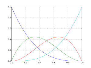
where the polynomials

are known as Bernstein basis polynomials of degree n.
Note that t0 = 1, (1 − t)0 = 1, and that the binomial coefficient, , also expressed as or , is:


The points Pi are called control points for the Bézier curve. The polygon formed by connecting the Bézier points with lines, starting with P0 and finishing with Pn, is called the Bézier polygon (or control polygon). The convex hull of the Bézier polygon contains the Bézier curve.
Polynomial form
Sometimes it is desirable to express the Bézier curve as a polynomial instead of a sum of less straightforward Bernstein polynomials. Application of the binomial theorem to the definition of the curve followed by some rearrangement will yield:

where

This could be practical if can be computed prior to many evaluations of ; however one should use caution as high order curves may lack numeric stability (de Casteljau's algorithm should be used if this occurs). Note that the empty product is 1.


Properties

- The curve begins at P0 and ends at Pn; this is the so-called endpoint interpolation property.
- The curve is a straight line if and only if all the control points are collinear.
- The start and end of the curve is tangent to the first and last section of the Bézier polygon, respectively.
- A curve can be split at any point into two subcurves, or into arbitrarily many subcurves, each of which is also a Bézier curve.
- Some curves that seem simple, such as the circle, cannot be described exactly by a Bézier or piecewise Bézier curve; though a four-piece cubic Bézier curve can approximate a circle (see composite Bézier curve), with a maximum radial error of less than one part in a thousand, when each inner control point (or offline point) is the distance horizontally or vertically from an outer control point on a unit circle. More generally, an n-piece cubic Bézier curve can approximate a circle, when each inner control point is the distance from an outer control point on a unit circle, where t is 360/n degrees, and n > 2.
- Every quadratic Bézier curve is also a cubic Bézier curve, and more generally, every degree n Bézier curve is also a degree m curve for any m > n. In detail, a degree n curve with control points P0, …, Pn is equivalent (including the parametrization) to the degree n + 1 curve with control points P'0, …, P'n + 1, where .
- Bézier curves have the variation diminishing property. What this means in intuitive terms is that a Bézier curves does not "undulate" more than the polygon of its control points, and may actually "undulate" less than that.[6]
- There is no local control in degree n Bézier curves—meaning that any change to a control point requires recalculation of and thus affects the aspect of the entire curve, "although the further that one is from the control point that was changed, the smaller is the change in the curve."[7]


Second order curve is a parabolic segment
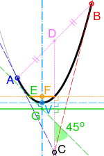
A quadratic Bézier curve is also a segment of a parabola. As a parabola is a conic section, some sources refer to quadratic Béziers as "conic arcs".[4] With reference to the figure on the right, the important features of the parabola can be derived as follows:[8]
- Tangents to the parabola at the end-points of the curve (A and B) intersect at its control point (C).
- If D is the midpoint of AB, the tangent to the curve which is perpendicular to CD (dashed cyan line) defines its vertex (V). Its axis of symmetry (dash-dot cyan) passes through V and is perpendicular to the tangent.
- E is either point on the curve with a tangent at 45° to CD (dashed green). If G is the intersection of this tangent and the axis, the line passing through G and perpendicular to CD is the directrix (solid green).
- The focus (F) is at the intersection of the axis and a line passing through E and perpendicular to CD (dotted yellow). The latus rectum is the line segment within the curve (solid yellow).
Derivative
The derivative for a curve of order n is

Constructing Bézier curves
Linear curves
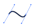
 |
| Animation of a linear Bézier curve, t in [0,1] |
The t in the function for a linear Bézier curve can be thought of as describing how far B(t) is from P0 to P1. For example, when t=0.25, B(t) is one quarter of the way from point P0 to P1. As t varies from 0 to 1, B(t) describes a straight line from P0 to P1.
Quadratic curves
For quadratic Bézier curves one can construct intermediate points Q0 and Q1 such that as t varies from 0 to 1:
- Point Q0(t) varies from P0 to P1 and describes a linear Bézier curve.
- Point Q1(t) varies from P1 to P2 and describes a linear Bézier curve.
- Point B(t) is interpolated linearly between Q0(t) to Q1(t) and describes a quadratic Bézier curve.
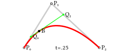 |  | |
| Construction of a quadratic Bézier curve | Animation of a quadratic Bézier curve, t in [0,1] |
Higher-order curves
For higher-order curves one needs correspondingly more intermediate points. For cubic curves one can construct intermediate points Q0, Q1, and Q2 that describe linear Bézier curves, and points R0 & R1 that describe quadratic Bézier curves:
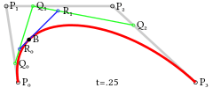 |  | |
| Construction of a cubic Bézier curve | Animation of a cubic Bézier curve, t in [0,1] |
For fourth-order curves one can construct intermediate points Q0, Q1, Q2 & Q3 that describe linear Bézier curves, points R0, R1 & R2 that describe quadratic Bézier curves, and points S0 & S1 that describe cubic Bézier curves:
 |  | |
| Construction of a quartic Bézier curve | Animation of a quartic Bézier curve, t in [0,1] |
For fifth-order curves, one can construct similar intermediate points.
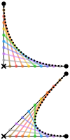
 |
| Animation of a fifth-order Bézier curve, t in [0,1] in red. The Bézier curves for each of the lower orders is also shown. |
These representations rest on the process used in De Casteljau's algorithm to calculate Bézier curves.[9]
Offsets (a.k.a. stroking) of Bézier curves
The curve at a fixed offset from a given Bézier curve, called an offset or parallel curve in mathematics (lying "parallel" to the original curve, like the offset between rails in a railroad track), cannot be exactly formed by a Bézier curve (except in some trivial cases). In general, the two-sided offset curve of a cubic Bézier is a 10th-order algebraic curve[10] and more generally for a Bézier of degree n the two-sided offset curve is an algebraic curve of degree 4n-2.[11] However, there are heuristic methods that usually give an adequate approximation for practical purposes.[12]
In the field of vector graphics, painting two symmetrically distanced offset curves is called stroking (the Bézier curve or in general a path of several Bézier segments).[10] The conversion from offset curves to filled Bézier contours is of practical importance in converting fonts defined in METAFONT, which allows stroking of Bézier curves, to the more widely used PostScript type 1 fonts, which only allow (for efficiency purposes) the mathematically simpler operation of filling a contour defined by (non-self-intersecting) Bézier curves.[13]
Degree elevation
A Bézier curve of degree n can be converted into a Bézier curve of degree n + 1 with the same shape. This is useful if software supports Bézier curves only of specific degree. For example, systems that can only work with cubic Bézier curves can implicitly work with quadratic curves by using their equivalent cubic representation.
To do degree elevation, we use the equality . Each component is multiplied by (1 − t) and t, thus increasing a degree by one, without changing the value. Here is the example of increasing degree from 2 to 3.


For arbitrary n we use equalities

introducing arbitrary and .


Therefore, new control points are [14]

Repeated Degree Elevation
The concept of Degree Elevation can be repeated on a control polygon R to get a sequence of control polygons R,R1,R2, and so on. After r degree elevations, the polygon Rr has the vertices P0,r,P1,r,P2,r,...,Pn+r,r given by [14]

It can also be shown that for the underlying Bézier curve B,

Rational Bézier curves
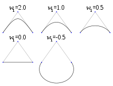
The rational Bézier curve adds adjustable weights to provide closer approximations to arbitrary shapes. The numerator is a weighted Bernstein-form Bézier curve and the denominator is a weighted sum of Bernstein polynomials. Rational Bézier curves can, among other uses, be used to represent segments of conic sections exactly, including circular arcs.[15]
Given n + 1 control points Pi, the rational Bézier curve can be described by:

or simply

See also
- Bézier surface
- B-spline
- Hermite curve
- NURBS
- String art – Bézier curves are also formed by many common forms of string art, where strings are looped across a frame of nails.
- Variation diminishing property of Bézier curves
Notes
- ↑ Image manipulation programs such as Inkscape, Adobe Photoshop, and GIMP.
- ↑ In animation applications such as Adobe Flash, Adobe After Effects, Microsoft Expression Blend, Blender, Autodesk Maya and Autodesk 3ds max.
References
- ↑ Biswas, Pradipta; Langdon, Pat (2015-04-03). "Multimodal Intelligent Eye-Gaze Tracking System". International Journal of Human-Computer Interaction. 31 (4): 277–294. doi:10.1080/10447318.2014.1001301. ISSN 1044-7318.
- ↑ Gerald E. Farin; Josef Hoschek; Myung-Soo Kim (2002). Handbook of Computer Aided Geometric Design. Elsevier. pp. 4–6. ISBN 978-0-444-51104-1.
- ↑ http://www.xlrotor.com/resources/files.shtml
- 1 2 FreeType Glyph Conventions, David Turner + Freetype Development Team, Freetype.org, retr May 2011
- ↑ John Burkardt. "Forcing Bezier Interpolation (from web.archive.org 2013-12-25)".
- ↑ Teofilo Gonzalez; Jorge Diaz-Herrera; Allen Tucker (2014). Computing Handbook, Third Edition: Computer Science and Software Engineering. CRC Press. page 32-14. ISBN 978-1-4398-9852-9.
- ↑ Max K. Agoston (2005). Computer Graphics and Geometric Modelling: Implementation & Algorithms. Springer Science & Business Media. p. 404. ISBN 978-1-84628-108-2.
- ↑ Duncan Marsh, Applied Geometry for Computer Graphics and CAD, Springer Undergraduate Mathematics Series, 2005
- ↑ Shene, C.K. "Finding a Point on a Bézier Curve: De Casteljau's Algorithm". Retrieved 6 September 2012.
- 1 2 http://www.slideshare.net/Mark_Kilgard/22pathrender, p. 28
- ↑ particularly p. 16 "taxonomy of offset curves"
- ↑ For example: or . For a survey see .
- ↑ MetaFog: Converting Metafont shapes to contours
- 1 2 Farin, Gerald (1997). Curves and surfaces for computer-aided geometric design (4 ed.). Elsevier Science & Technology Books. ISBN 978-0-12-249054-5
- ↑ Neil Dodgson (2000-09-25). "Some Mathematical Elements of Graphics: Rational B-splines". Retrieved 2009-02-23.
- Rida T. Farouki, The Bernstein polynomial basis: A centennial retrospective, Computer Aided Geometric Design, Volume 29, Issue 6, August 2012, Pages 379–419, doi:10.1016/j.cagd.2012.03.001
- Paul Bourke: Bézier Surfaces (in 3D), http://local.wasp.uwa.edu.au/~pbourke/geometry/bezier/index.html
- Donald Knuth: Metafont: the Program, Addison-Wesley 1986, pp. 123–131. Excellent discussion of implementation details; available for free as part of the TeX distribution.
- Dr Thomas Sederberg, BYU Bézier curves, http://www.tsplines.com/resources/class_notes/Bezier_curves.pdf
- J.D. Foley et al.: Computer Graphics: Principles and Practice in C (2nd ed., Addison Wesley, 1992)
- Rajiv Chandel: "Implementing Bezier Curves in games"
Computer code
Further reading and external links
- A Primer on Bézier Curves — An open source online book explaining Bézier curves and associated graphics algorithms, with interactive graphics.
- Cubic Bezier Curves - Under the Hood (video) Video shows how computers render a cubic Bézier curve, by Peter Nowell
- From Bézier to Bernstein Feature Column from American Mathematical Society
- Hazewinkel, Michiel, ed. (2001), "Bézier curve", Encyclopedia of Mathematics, Springer, ISBN 978-1-55608-010-4
- Hartmut Prautzsch; Wolfgang Boehm; Marco Paluszny (2002). Bézier and B-Spline Techniques. Springer Science & Business Media. ISBN 978-3-540-43761-1.
- Jean Gallier (1999). Curves and Surfaces in Geometric Modeling: Theory and Algorithms. Morgan Kaufmann. Chapter 5. Polynomial Curves as Bézier Curves. This book is out of print and freely available from the author.
- Gerald E. Farin (2002). Curves and Surfaces for CAGD: A Practical Guide (5th ed.). Morgan Kaufmann. ISBN 978-1-55860-737-8.
- Weisstein, Eric W. "Bézier Curve". MathWorld.
- http://web.archive.org/web/20061202151511/http://www.fho-emden.de/~hoffmann/bezier18122002.pdf
- Ahn, Young Joon (2004). "Approximation of circular arcs and offset curves by Bézier curves of high degree". Journal of Computational and Applied Mathematics. 167 (2): 405–416. doi:10.1016/j.cam.2003.10.008.